Alternative Beta Strategies


Alternative beta strategies are fundamentally about building a portfolio that doesn’t depend on one or two asset classes going up.
Most traders underestimate the tail risk of their portfolios. It’s easy to think you own a diversified portfolio holding an S&P 500 fund, some international equities, maybe a bond fund. That eliminates idiosyncratic risk (i.e., the risk associated with any single issuer or sector), but they still own a massive bet on equity market beta.
That works a lot of the time, in bursts and in cycles, but when it doesn’t, the equity beta dominates and everything more or less goes down together.
Alternative beta is the answer to that problem. It’s not a single strategy, but a way of thinking about returns: the idea that markets pay you for taking certain kinds of risk, and that traditional market-cap indexing only captures one slice of the available risk premia.
The rest sit there for those willing to think in terms of factors, styles, and structural inefficiencies rather than just “the market.”
Let’s walk through how this actually works, what the trade-offs are, and how to put it to work in a real portfolio.
Key Takeaways – Alternative Beta Strategies
- Traditional portfolios feel diversified but are still one dominant bet (equities).
- Alternative beta reframes returns as multiple compensated risks.
- The edge is structural diversification across factors, which are essentially different beta constructions (value, momentum, quality, low vol, carry).
- The goal isn’t higher raw return, but smoother, more durable return streams.
- You’re not optimizing returns, but optimizing the reliability of returns across different unknown futures.
What Returns Actually Are
Before we get to alternative beta, you have to understand what any return actually consists of. I think of returns as having three components stacked on top of each other.
Risk-free rate
The first is the risk-free rate. This is what you get for parking cash in an instrument like 3-month Treasury bills. You aren’t taking any meaningful credit risk or market risk (no nominal price risk).
You’re being compensated for the time value of money and not much else. Costs exist in the form of inflation and taxes on the interest, so always factor that in.
Beta
The second is beta. Beta is what you earn for taking on systematic market risk.
If you own the S&P 500, your beta to the equity market is approximately 1.0, which means you go up and down with the market in roughly equal measure.
The long-run equity risk premium in the US has averaged about 5-6% over Treasuries. That premium exists because stocks are riskier than cash, and investors demand to be paid for holding them.
Equity risk varies over time and it could be true that the equity risk premium going forward is less than what it’s been historically.
Alpha
The third is alpha. Alpha is the return you generate above and beyond the market’s return, after accounting for the risk you took. Alpha is rare. It’s hard and zero-sum (negative-sum after transaction costs).
Most active managers don’t actually generate it after fees, which is why most are better off with low-cost index exposure than expensive active management.
“The Market” = Risk-free rate + Beta
Traditional indexing gives you risk-free rate plus market beta. That’s it. You’re collecting one risk premium: the equity risk premium.
But the academic and practitioner research over the last forty years has identified other risk premia, what most call alternative betas, that pay you for taking on different kinds of risk.
They aren’t alpha, because they’re systematic and rules-based. In other words, they’re known.
They aren’t traditional beta, because they don’t track the market-cap index. They sit in between.
That’s what we’ll look at.
What Alternative Beta Actually Is
Alternative beta strategies, sometimes called “smart beta,” try to capture risk premia beyond the standard market-cap index.
The vehicles look familiar (ETFs, index funds, mutual funds) but the construction is different. Instead of weighting holdings by market capitalization, alternative beta funds weight by some other characteristic that has historically been associated with excess returns.
Why does this work? Two reasons.
Structural
The first is structural. Some risk premia exist because investors must be compensated for genuine, persistent risks.
Small-cap stocks are more volatile and less liquid than large caps, so they pay a premium.
Value stocks are often distressed companies that bear real solvency risk, so they pay a premium.
The premium is the price the market charges for bearing that risk over time.
Behavioral
The second is behavioral. Investors systematically misprice certain securities because of well-documented biases.
They chase recent winners (which creates the momentum premium).
They overpay for glamorous growth stories (which creates the value premium).
They demand lottery-like upside in high-volatility stocks (which is why low-volatility stocks have historically outperformed on a risk-adjusted basis, despite the textbook saying they shouldn’t).
Both have been studied across decades of data and across many different markets, which gives me confidence they’re closer to “timeless and universal” and not just a fad or something that gets arbed out of markets when enough of the market wises up to them.
The Major Factors
Let me walk through what has the strongest empirical support.
Value
The classic factor, dating back to Graham and Dodd in the 1930s and formalized by Fama and French in the early 1990s.
The idea is straightforward: cheap stocks (measured by price-to-book, price-to-earnings, price-to-cash-flow) tend to outperform expensive stocks over long horizons.
Why? Partly because cheap companies bear more genuine financial risk. Partly because investors get bored of slow-growing businesses and overpay for exciting ones.
The premium has historically averaged 3-5% annually in US equities, but it goes through long stretches of underperformance.
The decade from roughly 2010 to 2020 was brutal for value investors. The premium came back hard in 2021-2022 when interest rates rose. That cyclicality is the price of admission.
Momentum
Stocks that have outperformed over the past 6-12 months tend to keep outperforming over the next 1-3 months.
Stocks that have underperformed tend to keep underperforming. This is one of the most robust findings in empirical finance, documented across stocks, bonds, currencies, commodities, and real estate, going back over a century.
Why does it work?
Traders and investors anchor on old information and react slowly to new information.
They also herd into what’s already working.
The premium is real but it pays in a way that makes it hard to stand by: long stretches of steady gains punctuated by sharp, painful crashes when the market regime shifts.
The 2009 momentum crash was one of the worst factor blow-ups on record.
Size
Small-cap stocks have outperformed large-cap stocks over very long horizons, by roughly 2% annually in the US.
The premium exists because small caps are more volatile, less liquid, more exposed to recession risk, and harder to research.
The size premium has weakened in recent decades, partly because more investors are aware of it and partly because the small-cap universe has changed.
In fact, this century, and especially since the 2008 financial crisis, the size premium has been negative. Most of the benefits have accrued to larger firms.
I’d treat it as real but not as strong as it once was.
Quality
Stocks of companies with strong balance sheets, high return on equity, low leverage, and stable earnings tend to outperform on a risk-adjusted basis.
This is the factor that explains why Warren Buffett’s track record looks like alpha but is actually mostly quality plus value plus modest leverage.
The quality premium is more behavioral than structural. Most market participants get excited about exciting stories and hence they underweight boring, profitable, well-run businesses.
Low volatility
This one is the most counterintuitive.
If you take finance in school, you learn that the textbook capital asset pricing model says higher-risk stocks should produce higher returns.
But the data says the opposite.
Low-volatility stocks have historically delivered equity-like returns with materially lower drawdowns.
Why? Because investors have a structural preference for high-volatility lottery tickets, leverage constraints push institutional money to chase return through high-beta stocks rather than leveraged low-beta stocks, and the demand for “boring” stocks is structurally lower than it should be.
The low-vol anomaly is one of the strongest factor signals on the data.
Carry
This is more relevant in fixed income, currencies, and commodities than in equities. Carry means earning a yield differential by holding higher-yielding assets and funding the position with lower-yielding ones.
The classic example is the FX carry trade: borrow in, e.g., yen (cheap), lend in, e.g., Australian dollars (higher rate), collect the rate differential.
Carry pays steadily for long periods and then loses a lot when risk aversion spikes. You collect pennies in front of a steamroller, but the pennies add up if you size the position correctly.
Others
These are the major risk premia.
There are others (profitability, investment, term premium, default premium, liquidity premium, betting against beta) but the six above cover most of what matters.
Briefly:
- Profitability – Companies with strong, stable profits tend to outperform weaker ones. Markets often underprice consistent earnings quality and capital efficiency
- Investment – Firms that invest conservatively tend to outperform aggressive expanders. High asset growth often signals overinvestment and lower future returns.
- Term Premium – The extra return demanded for holding longer-duration bonds due to interest rate risk and uncertainty about future inflation.
- Default Premium – Extra yield earned for taking on credit risk. Compensates investors for the probability and severity of borrower default.
- Liquidity Premium – Extra return required for holding harder-to-trade assets. Has to do with the cost and risk of not being able to exit positions.
- Betting Against Beta – Strategy that goes long low-beta assets and short high-beta ones.
The Practitioner View – Why This Matters
Each of these factors has similar risk-adjusted returns, but they’re not perfectly correlated with the equity market or with each other. Value can be down when momentum is up.
Quality can hold its ground when small-caps get hit. Low-volatility provides ballast in drawdowns.
If you can engineer exposure to multiple factors that have similar expected returns but different drivers, you reduce portfolio risk without sacrificing expected return.
That’s the alpha-beta separation. You’re not generating alpha by stock picking. You’re combining several different betas, each with their own risk premium, in a way that produces a smoother return stream than any one of them alone.
You aren’t trying to beat the market through cleverness or figuring things out that other professional traders and investors haven’t – which is essentially what alpha is. You’re trying to harvest multiple, partially uncorrelated return streams and let the diversification do the work.
Multi-Factor: Why Combination Beats Concentration
Single-factor portfolios are dangerous. Value goes through ten-year+ droughts. Momentum has spectacular crashes. Size paid negatively for more than two decades – a timeframe when most would start to consider whether it even exists or the opposite is true.
If you bet on one factor and it’s the wrong decade, you’ll underperform the market by enough to make you give up at the worst possible moment.
Multi-factor strategies fix this by combining factors with different cyclical patterns. The combinations that have shown the strongest empirical support are:
- Value plus momentum (negatively correlated, smooths the ride)
- Value plus quality (the “Buffett portfolio“)
- Quality plus low volatility (the “sleep at night” combination)
- Value plus momentum plus quality plus low volatility (the kitchen-sink approach)
A simple equal-weighted combination of value, momentum, quality, and low-volatility factors has historically delivered better risk-adjusted returns than any single factor and better than the market itself.
Not because any one factor is special, but because the diversification across factors does what diversification is supposed to do.
How Factors Behave Across Macro Environments
This is the part of factor investing that most academic literature underweights and that I think is the most important for a trader or investor in 2026.
Factors are driven by the same forces that drive everything else in markets: the debt cycle, monetary policy, growth, inflation, and the relationships between them.
If you understand how each factor responds to different macro environments, you can think about your factor exposure the same way you think about your asset allocation: balanced across the conditions you’ll actually live through.
Value loves rising rates and rising inflation
Value stocks tend to be cyclical businesses with near-term cash flows: banks, energy producers, utilities, industrial companies, consumer staples with pricing power.
When real rates rise, the present value of long-duration growth stocks drops faster than the present value of value stocks, because the growth stocks’ cash flows are further out in time.
This is exactly what happened in 2022, when the Fed raised rates aggressively and the Russell 1000 Value beat the Russell 1000 Growth by roughly 20 percentage points in a single year.
Value also tends to do well in inflationary environments because value companies often have physical assets and short-duration cash flows that reprice with inflation.
If you think we’re in a higher-for-longer rate environment, value should be overweighted in your factor mix.
Momentum loves trending markets and hates regime changes
Momentum works in any market that trends, up or down, for long enough that the recent past predicts the near future.
It tends to fail terribly at inflection points, when the market changes regime and yesterday’s winners become tomorrow’s losers.
The 2009 momentum crash happened because the strategy was short the worst-performing financials going into March 2009 and then those same financials rallied 200%-plus when the credit panic ended.
The 2022 momentum reversal happened because momentum was long expensive growth stocks at the top and got destroyed when rates rose.
As a trader, you should expect momentum to do well during long expansions and to take losses during turning points. The premium is the price you pay for owning the wrong thing at exactly the wrong moment, occasionally.
Quality loves recessions and ugly markets
Quality companies have strong balance sheets, low debt, high margins, and stable earnings.
They don’t outperform much during exuberant bull markets because investors aren’t worried about solvency or earnings stability.
They do outperform during recessions and credit contractions because that’s when the strength of the balance sheet starts to matter.
In 2008-2009, quality outperformed the S&P 500 by roughly 10 percentage points. In the COVID drawdown of March 2020, quality held up materially better than the index.
Quality is your factor for the late-cycle and recession environments. It’s the factor that performs when policymakers are doing the “four levers” (namely austerity, defaults, money printing, and wealth transfers) suboptimally.
Low volatility loves drawdowns and disinflation
Low-volatility stocks have historically been concentrated in utilities, consumer staples, healthcare, and related defensive sectors.
They benefit from falling rates because they’re bond-like in their cash flow profile. They benefit from drawdowns because they fall less than the market.
They underperform during sharp recoveries (because they don’t bounce as hard) and during inflationary periods (because their long-duration cash flows are penalized by rising rates). The 2010-2019 environment of falling rates and low inflation was nearly ideal for low volatility.
The 2022 environment of rising rates was much harder.
Carry loves stable, low-volatility regimes and gets crushed in crises
This is most relevant in fixed income and currencies, less so in equities.
Carry pays steadily as long as nothing breaks and then loses violently when something does.
The 2008 unwind of the FX carry trade, when the yen rallied 30% against the Australian dollar in a few months, is the textbook example.
Carry is a great strategy if you can size it correctly and accept that you’ll have crisis-period losses.
So how does this map to portfolio construction? The same way it does for asset allocation. You don’t try to time which factor will work next year.
You hold a balanced exposure to factors that perform in different environments, accept that some will be underperforming at any given time, and let the portfolio-level diversification reduce the volatility of your overall return stream.
Said differently: factor diversification within equities works for the same reason that asset class diversification works across the portfolio.
Different drivers, different cyclical patterns, different responses to the same macro shocks.
The goal isn’t to predict which one will be the best. It’s to own enough of each that the portfolio doesn’t depend on any single bet.
How to Actually Implement This
There are three practical paths.
Single-factor ETFs
Vanguard, iShares, and Invesco all offer factor ETFs at low fees, typically 15-30 basis points (i.e., for every $10,000 invested, it comes with $15-$30 in annual fees).
You can build a multi-factor portfolio by combining several of these.
The advantage is transparency and control. The disadvantage is that you have to rebalance across them and the factor definitions vary.
Multi-factor ETFs
Funds like iShares MSCI USA Multifactor (LRGF), Goldman Sachs ActiveBeta (GSLC), and various offerings from Dimensional, AQR, and Research Affiliates package multiple factors into a single vehicle.
Fees run 25-45 basis points. You give up some control over factor weighting but gain simplicity.
Direct indexing
For investors with $100,000-plus and the right tax situation, direct indexing platforms (Wealthfront, Schwab, Frec, and others) let you own the underlying stocks directly with factor tilts and tax-loss harvesting. This is the most flexible but also the most complex.
For most people, a combination of two or three multi-factor ETFs will get you the bulk of the benefit without the complexity. The diminishing returns to portfolio sophistication are real.
What These Strategies Actually Look Like in Practice
Let me make this concrete with three example trades. Assume a $100,000 portfolio.
Trade 1: Value Factor Tilt
Objective = capture the value premium by owning stocks that look cheap on traditional valuation metrics.
Screen for stocks with price-to-earnings below 15 and price-to-book below 1.5, in the largest 1,000 US-listed companies. Rank by composite cheapness score. Take the top 30.
Position size = 3.3% per name, $3,333 each. Rebalance quarterly. Target turnover roughly 30-40% per year.
What you should expect – Long-run excess return over the S&P 500 of perhaps 2-4% annualized, with tracking error of 5-8% and stretches of 3-5 year underperformance during growth-led markets. The strategy will look bad in markets like 2017-2019 and much better in markets like 2022. If you can’t sit through the bad years, don’t run the strategy.
Trade 2: Momentum Factor Tilt
Objective = ride trends in stocks that have been outperforming.
Screen for stocks in the largest 1,000 US-listed companies. Rank by 12-month total return excluding the most recent month (the standard academic definition, which avoids short-term reversal). Take the top 30.
Position size = 3.3% per name, $3,333 each. Rebalance monthly. Target turnover of 200-400% per year, which means you need to hold this in a tax-advantaged account or accept the tax drag.
What you should expect – long-run excess return of 4% annualized, but with occasional momentum crashes that can take the strategy down 30%-plus in a few months. The 2009 momentum crash and the 2022 momentum reversal are recent examples. The premium is real but the path is rough.
Trade 3: Low-Volatility Factor Tilt
Objective = get equity-like returns with materially lower drawdowns.
Screen for stocks with the lowest realized volatility over the trailing 12 months in the largest 1,000 US-listed companies. Apply quality screens (positive earnings, reasonable leverage). Take the lowest-volatility 30 names.
Position size = 3.3% per name, $3,333 each. Rebalance semi-annually.
What you should expect – returns roughly in line with the S&P 500 over full cycles but with 15-20% lower volatility and meaningfully smaller drawdowns. The strategy underperforms in fast recoveries (2009, 2020) and outperforms in drawdowns (2008, 2022). Sharpe ratio improvement is the goal, not absolute outperformance. Some more advanced traders lever up to the intended volatility to achieve better absolute return.
These are illustrative. In a real portfolio, I would not run any of these as standalone bets. I would combine them.
A Multi-Factor Combination
Take that same $100,000 and split it as follows:
- $25,000 in value factor exposure
- $25,000 in momentum factor exposure
- $25,000 in quality factor exposure
- $25,000 in low-volatility factor exposure
The historical record on this kind of equal-weighted multi-factor portfolio shows excess returns of 1-3% over the S&P 500 with similar or lower drawdowns and a much smoother return profile. You’re not trying to win big, but win more consistently.
Where Alternative Beta Fits in a Real Portfolio
Fundamentally, it’s a refinement within the equity portion of a properly diversified portfolio.
The first job of portfolio construction is to balance exposure to the major economic environments: rising growth, falling growth, rising inflation, falling inflation – all relative to expectation.
You hold assets that perform in each environment in roughly risk-balanced proportions.
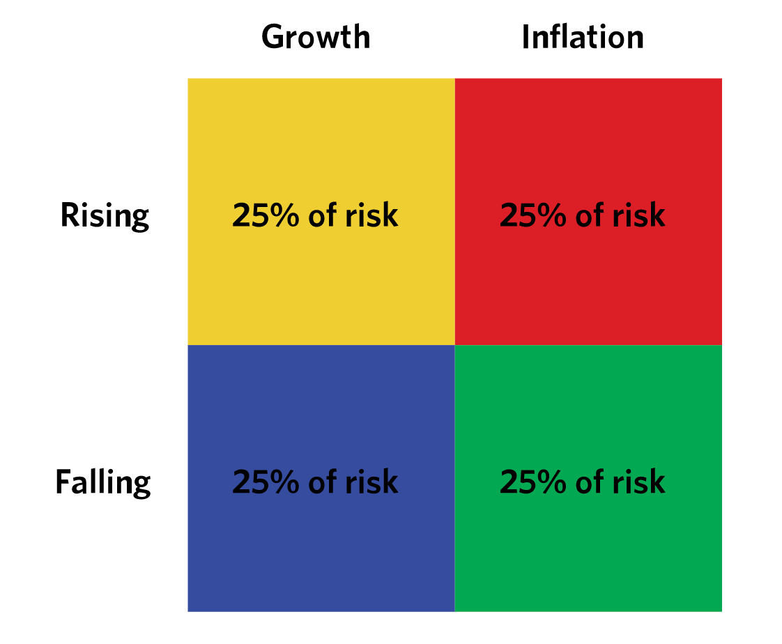
- Stocks for rising growth.
- Long bonds for falling growth.
- Commodities for rising inflation.
- Inflation-linked bonds for positive inflation and falling growth (relative to nominal bonds).
For example:
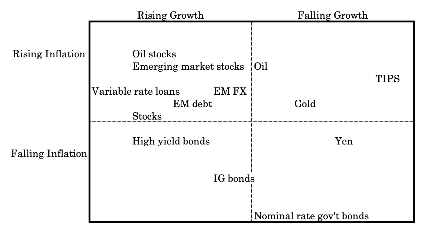
Once you have that strategic asset allocation right, then you can think about how to express the equity portion of it.
Within your equity allocation, you can choose to hold market-cap index, or you can tilt toward value, momentum, quality, low-volatility, or some combination.
The factor decision is a second-order optimization on top of the first-order asset allocation decision.
The main idea = don’t run a 100% equity factor portfolio and call it diversified. It isn’t. It’s still 100% equity beta with some factor tilts on top. Real diversification comes from owning genuinely different return streams. Factors help, but they don’t substitute for asset allocation.
Factor Statistics
We have a fuller article on factor statistics located here.
Here, we’re going to take a look at correlations, return, and volatility of the various things we’ve been talking about:
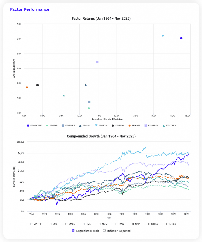
Fama-French Research Factors
| Factor | Key | Rm-Rf | SMB | SMB5 | HML | MOM | RMW | CMA | STREV | LTREV | Annualized Return | Annualized Standard Deviation |
|---|---|---|---|---|---|---|---|---|---|---|---|---|
| Market | FF-MKT-RF | 1.00 | 0.30 | 0.28 | -0.21 | -0.17 | -0.19 | -0.35 | 0.30 | -0.01 | 6.04% | 15.50% |
| Size (FF3) | FF-SMB | 0.30 | 1.00 | 0.98 | -0.14 | -0.05 | -0.40 | -0.17 | 0.17 | 0.25 | 1.32% | 10.51% |
| Size (FF5) | FF-SMB5 | 0.28 | 0.98 | 1.00 | 0.01 | -0.08 | -0.34 | -0.08 | 0.17 | 0.32 | 1.74% | 10.53% |
| Value | FF-HML | -0.21 | -0.14 | 0.01 | 1.00 | -0.20 | 0.09 | 0.68 | 0.02 | 0.52 | 2.90% | 10.33% |
| Momentum | FF-MOM | -0.17 | -0.05 | -0.08 | -0.20 | 1.00 | 0.08 | -0.01 | -0.30 | -0.09 | 6.15% | 14.51% |
| Profitability | FF-RMW | -0.19 | -0.40 | -0.34 | 0.09 | 0.08 | 1.00 | 0.01 | -0.07 | -0.26 | 2.87% | 7.72% |
| Investment | FF-CMA | -0.35 | -0.17 | -0.08 | 0.68 | -0.01 | 0.01 | 1.00 | -0.13 | 0.51 | 2.72% | 7.17% |
| Short Term Reversal | FF-STREV | 0.30 | 0.17 | 0.17 | 0.02 | -0.30 | -0.07 | -0.13 | 1.00 | 0.10 | 4.44% | 10.96% |
| Long Term Reversal | FF-LTREV | -0.01 | 0.25 | 0.32 | 0.52 | -0.09 | -0.26 | 0.51 | 0.10 | 1.00 | 2.18% | 9.15% |
| Factor correlations and returns statistics from January 1964 to November 2025 | ||||||||||||
Market and momentum see the highest returns. Momentum gives strong performance but high vol/variance in outcomes.
Value, profitability, and investment provide moderate returns with lower risk and useful diversification (due to low/negative correlations with the market).
Size effects are modest. Reversal factors offer diversification benefits but weaker standalone returns.
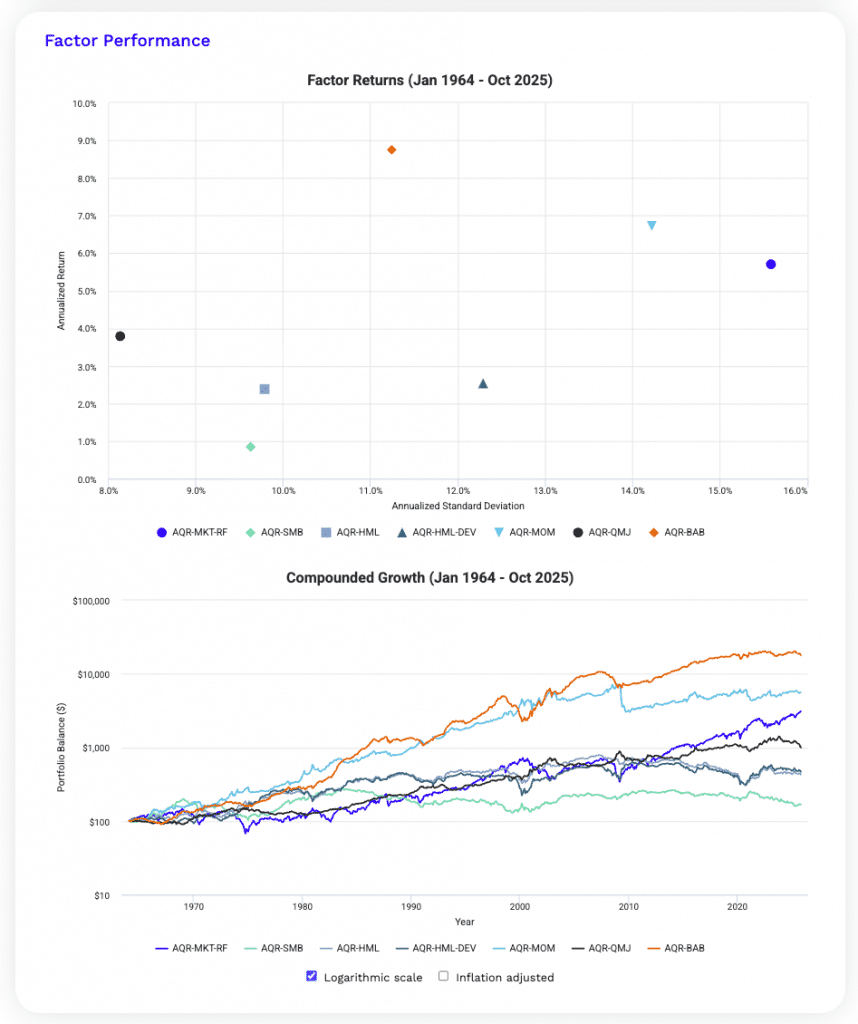
AQR Factors
Factor Correlations
| Factor | Key | Rm-Rf | SMB | HML | HML-DEV | MOM | QMJ | BAB | Annualized Return | Annualized Standard Deviation |
|---|---|---|---|---|---|---|---|---|---|---|
| Market | AQR-MKT-RF | 1.00 | 0.31 | -0.23 | -0.06 | -0.19 | -0.53 | -0.09 | 5.71% | 15.58% |
| Size | AQR-SMB | 0.31 | 1.00 | -0.07 | 0.02 | -0.14 | -0.51 | -0.04 | 0.85% | 9.63% |
| Value | AQR-HML | -0.23 | -0.07 | 1.00 | 0.79 | -0.14 | -0.06 | 0.36 | 2.39% | 9.79% |
| Value | AQR-HML-DEV | -0.06 | 0.02 | 0.79 | 1.00 | -0.64 | -0.23 | 0.12 | 2.53% | 12.29% |
| Momentum | AQR-MOM | -0.19 | -0.14 | -0.14 | -0.64 | 1.00 | 0.31 | 0.21 | 6.73% | 14.22% |
| Quality | AQR-QMJ | -0.53 | -0.51 | -0.06 | -0.23 | 0.31 | 1.00 | 0.20 | 3.79% | 8.14% |
| Bet Against Beta | AQR-BAB | -0.09 | -0.04 | 0.36 | 0.12 | 0.21 | 0.20 | 1.00 | 8.75% | 11.25% |
| Factor correlations and returns statistics from January 1964 to October 2025 | ||||||||||
AQR factors show momentum and bet-against-beta (BAB) as the strongest return drivers. BAB gives the highest risk-adjusted performance.
Quality gives good returns with low volatility and strong defensive properties, which shows in negative market correlation.
Value and value-deviation are highly correlated but cyclical, while size contributes little in return on their own.
So, overall, diversification benefits come mainly from quality, momentum, and BAB.
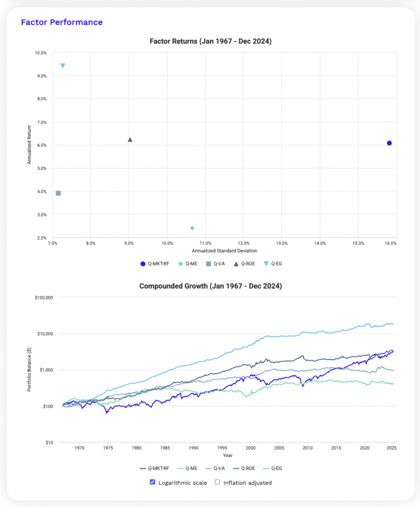
q-Factors
Factor Correlations
| Factor | Key | Rm-Rf | ME | I/A | ROE | EG | Annualized Return | Annualized Standard Deviation |
|---|---|---|---|---|---|---|---|---|
| Market | Q-MKT-RF | 1.00 | 0.28 | -0.35 | -0.22 | -0.43 | 6.08% | 15.82% |
| Size | Q-ME | 0.28 | 1.00 | -0.09 | -0.32 | -0.41 | 2.40% | 10.66% |
| Investment | Q-I/A | -0.35 | -0.09 | 1.00 | 0.05 | 0.18 | 3.92% | 7.15% |
| Return on Equity | Q-ROE | -0.22 | -0.32 | 0.05 | 1.00 | 0.53 | 6.23% | 9.03% |
| Expected Growth | Q-EG | -0.43 | -0.41 | 0.18 | 0.53 | 1.00 | 9.42% | 7.26% |
| Factor correlations and returns statistics from January 1967 to December 2024 | ||||||||
Expected growth and ROE deliver the highest returns with moderate volatility and strong correlation.
Investment offers defensive diversification via negative market exposure.
Size is modest.
Overall, profitability and growth dominate risk-adjusted performance.
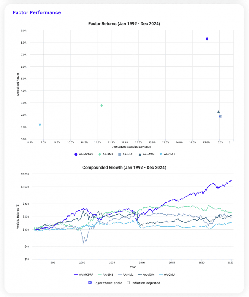
Alpha Architects
Factor Correlations
| Factor | Key | Rm-Rf | SMB | HML | MOM | QMJ | Annualized Return | Annualized Standard Deviation |
|---|---|---|---|---|---|---|---|---|
| Market | AA-MKT-RF | 1.00 | 0.27 | -0.32 | -0.25 | -0.34 | 8.28% | 15.03% |
| Size | AA-SMB | 0.27 | 1.00 | -0.27 | -0.19 | -0.40 | 2.75% | 11.15% |
| Value | AA-HML | -0.32 | -0.27 | 1.00 | -0.30 | 0.12 | 1.87% | 15.52% |
| Momentum | AA-MOM | -0.25 | -0.19 | -0.30 | 1.00 | 0.73 | 2.26% | 15.46% |
| Quality | AA-QMJ | -0.34 | -0.40 | 0.12 | 0.73 | 1.00 | 1.15% | 8.87% |
| Factor correlations and returns statistics from January 1992 to December 2024 | ||||||||
Alpha Architect factors show modest premia outside the market.
Momentum and quality are highly correlated, which limit diversification.
Value and size underperform with higher volatility.
Returns are driven primarily by market exposure.
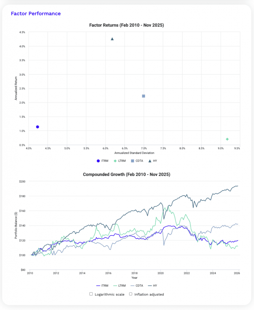
Fixed Income Factors
Factor Correlations
| Factor | Key | ITRM | LTRM | CDT | HY | Annualized Return | Annualized Standard Deviation |
|---|---|---|---|---|---|---|---|
| Intermediate Term Rate Risk | ITRM | 1.00 | 0.73 | 0.06 | 0.00 | 1.13% | 4.23% |
| Long Term Rate Risk | LTRM | 0.73 | 1.00 | -0.03 | -0.11 | 0.70% | 9.17% |
| Credit Risk | CDTA | 0.06 | -0.03 | 1.00 | 0.87 | 2.23% | 6.99% |
| High Yield Credit Risk | HY | 0.00 | -0.11 | 0.87 | 1.00 | 4.26% | 6.17% |
| Factor correlations and returns statistics from February 2010 to November 2025 | |||||||
Fixed income returns are driven by credit, especially high yield.
Rate risk offers lower returns and diversification.
What Can Go Wrong
You should think hard about what can break each of these strategies.
Crowding
When too many traders/investors pile into a factor, the factor’s premium gets compressed.
The decade of value underperformance from 2010-2020 was partly a crowding problem: everyone read the academic papers, everyone bought value ETFs, and the premium got temporarily arbitraged away. It came back, but it took a long time.
If a factor has $500 billion of capital chasing it, the next 10 years of returns will probably be lower than the historical record.
Regime change
Factors that worked in one monetary regime can fail in another.
Low volatility loved the post-2008 zero-rate environment because investors were starved for any kind of yield-like return.
Momentum loved the trending markets of 2003-2007 and 2010-2019 and got crushed when those trends reversed. The factor that worked best in the last decade is rarely the one that works best in the next.
Implementation
Factor definitions matter.
A “value” ETF that uses price-to-book will own different stocks than one using free cash flow yield.
A “quality” ETF that emphasizes return on equity will look different from one using earnings stability.
These differences compound. Read the prospectus and understand what you actually own.
Tax drag
High-turnover factor strategies (momentum especially) generate short-term capital gains that get taxed at ordinary income rates.
In a taxable account, a momentum strategy that delivers 8% gross might deliver 5% after taxes. That changes the math considerably.
Behavioral risk
This is the biggest risk and the one nobody talks about. Factor strategies underperform the market for years at a time.
If you can’t hold the strategy through the bad years, you’ll sell at the bottom and miss the recovery.
The historical premiums assume you held through every drawdown. Most investors don’t. The premium is the price you pay for sitting in your seat when everyone else is running.
What I Would Actually Do
If I had $100,000 to manage and I’m thinking about how to think about this, here’s roughly what I’d say.
Start with the asset allocation question first.
Decide what percentage of your portfolio should be in equities, bonds, real assets, and cash, and balance that allocation across the four major economic environments (i.e., rising/falling growth/inflation). That decision drives ~80% of your long-run outcome.
Within the equity part, default to a low-cost market-cap index unless you have a specific reason to tilt. For example, if you want less volatility and more stable cash flows, then tilt toward more defensive sectors like consumer staples, utilities, and healthcare.
The market-cap index isn’t optimal, but it’s not bad, and the simplicity has value.
If you want to add factor exposure, start with a single multi-factor ETF that combines value, quality, and momentum at low cost. Avoid single-factor concentration unless you have very strong conviction and a long horizon.
Size the factor tilt to a fraction of the equity portion. Don’t put the whole portfolio on it.
The factor premia work over longer horizons. Looking at them on a quarterly basis will only convince you to abandon them at the worst possible time.
Match the strategy to the account type. High-turnover factors go in IRAs and 401(k)s. Low-turnover factors and broad market exposure can sit in taxable accounts.
Be honest with yourself about your willingness to hold a factor through years of underperformance. If you’ll capitulate during the bad years, the premium isn’t there for you, no matter what the historical record says.
The Big Picture
Alternative beta is one of the most important developments in retail and institutional portfolio management of the last thirty years.
It democratizes what were once proprietary quantitative strategies and makes them available at low cost.
It gives you a way to think about returns that goes beyond “the market went up” or “the market went down.”
The big picture arc is this: markets pay you for taking risk, but they pay different prices for different kinds of risk.
Some of those risks are well-known (equity beta, term premium, credit spread).
Others are less appreciated (value, momentum, quality, low volatility, carry).
The trader who understands the full range of compensated risks and combines them thoughtfully will produce a smoother, more durable return stream than the investor who concentrates in just one.
That doesn’t make alternative beta a magic solution. The premia are real but variable. The strategies require patience.
The implementation matters. And no amount of factor sophistication substitutes for getting the asset allocation right in the first place.
But for an investor willing to think carefully about how returns are actually generated, alternative beta is one of the most important tools available.
Use it correctly and it will compound for you over decades. Use it badly and it will give you another way to lose money. The difference is in the thinking.
In the end, the goal isn’t to find the cleverest strategy. It’s to build a portfolio that performs across the environments you’ll actually live through, at a cost you can afford, with a structure you can actually stick with.
Alternative beta, used thoughtfully alongside proper asset allocation, gets you closer to that goal than market-cap indexing alone.
That’s the real edge. Not cleverness. Discipline plus diversification, applied across multiple risk premia, held through the cycles. The math takes care of the rest.