Stochastic Optimal Control in Finance

Stochastic Optimal Control represents a mathematical framework used to determine optimal decision-making strategies in situations where outcomes are:

• partly random, and
• partly under the control of a decision-maker (e.g., trading, investing, financial decision-making)

This concept is rooted in the theory of stochastic processes and optimal control theory.

Stochastic Process

A stochastic process is a mathematical object that represents a sequence of random variables evolving over time according to certain probabilistic rules.

Optimal Control Theory

Optimal control theory is a branch of mathematics that deals with finding a control law for a dynamical system over time such that a certain objective (usually expressed as a cost or utility function) is optimized.

Key Takeaways – Stochastic Optimal Control

• Dynamic Decision Making:
  • Stochastic Optimal Control is used for making decisions in uncertain environments.
  • It aids in determining the best course of action by considering the stochastic (“random”) nature of the environment and the future states of the system.
• Applications in Finance:
  • This technique can be used for portfolio optimization, option pricing, and risk management.
  • Adapts strategies dynamically to market conditions.
• Mathematics:
  • The field involves mathematical concepts like stochastic processes, partial differential equations, and dynamic programming.

Example of Optimal Control Theory in Finance

A pertinent example of optimal control theory is the dynamic asset allocation problem in portfolio management.

Here, the objective is to maximize the expected return of a portfolio over a given time horizon while managing risk, often quantified as portfolio variance or Value at Risk (VaR).

In this scenario, the dynamical system is the portfolio.

Its state is defined by the allocation of assets (like stocks, bonds, and cash) and their respective values, which evolve over time according to market dynamics.

The control law in this context is the strategy for reallocating assets in the portfolio over time.

The objective function could be to maximize the expected return of the portfolio for a given level of risk or to minimize risk for a given level of expected return.

Optimal control theory helps in determining how and when to rebalance the portfolio, taking into consideration factors like transaction costs, market impact, liquidity constraints, and changing market conditions.

The theory provides a framework to formulate and solve this problem.

It often involves stochastic differential equations to model asset price dynamics and techniques like dynamic programming or Monte Carlo simulations for solving the control problem.

In finance, the fusion of stochastic control theory is exemplified in the management of an investment portfolio under uncertain market conditions.

This complex problem involves dynamically adjusting the portfolio’s asset allocation to maximize expected returns or utility while minimizing risk, considering the stochastic (“random”) nature of financial markets.

Example: Optimal Portfolio Rebalancing Under Uncertainty

Stochastic Process

The prices of financial assets (stocks, bonds, etc.) in the portfolio are modeled as stochastic processes, often using Geometric Brownian Motion or other models that capture the random walk nature of market prices.

Dynamical System

The state of the system is the current allocation of assets in the portfolio, including the cash position, and their market values, which change over time based on market dynamics and the trader’s actions.

Control Law

The trader’s decision on how to rebalance the portfolio – buying or selling assets – at different points in time.

This decision is based on a strategy that seeks to optimize a specific objective (e.g., maximize return at a certain volatility level).

Objective Function

Typically, the goal is to maximize the expected utility of final portfolio value.

This incorporates both the expected returns and the risk (often measured by variance or a similar metric).

Alternatively, the objective might be to achieve a certain level of return while minimizing risk.

Optimization under Uncertainty

The trader needs to consider not only the current state of the market but also potential future states.

Stochastic control theory provides a framework for making optimal decisions in this environment.

Mathematical Tools

Techniques such as Stochastic Dynamic Programming or the Hamilton-Jacobi-Bellman (HJB) equation might be employed to solve such problems.

These tools help in deriving the optimal policy – rules for when and how to rebalance the portfolio given the current market state and the predicted stochastic evolution of asset prices.

Key Considerations

• Risk-Return Trade-Off: The trader needs to consider how much risk is acceptable for the anticipated return. This risk aversion is typically encoded in the utility function.
• Market Impact and Transaction Costs: Real-world factors like the impact of large trades on market prices and the costs associated with buying and selling assets must be factored into the model.
• Regulatory and Operational Constraints: These may include liquidity requirements, regulatory limits on certain types of investments, and other operational constraints.

Other Applications in Finance, Trading, and Investing

Portfolio Optimization

In the context of portfolio management, Stochastic Optimal Control is used to dynamically allocate assets in a way that maximizes expected utility, considering the stochastic nature of asset returns.

It extends the classical Markowitz portfolio theory by incorporating dynamic rebalancing in response to market changes.

Risk Management

This approach is used to model and manage risk in financial portfolios.

It can optimize the trade-off between risk and return by considering the stochastic nature of market risks and the dynamic aspect of risk management strategies.

Option Pricing and Hedging

Stochastic Optimal Control plays a key role in the pricing of financial derivatives, particularly options.

The famous Black-Scholes-Merton model, a cornerstone of modern financial theory, is an application of this concept.

It also informs dynamic hedging strategies, where the hedge ratio is adjusted in response to market movements.

Asset-Liability Management

In banking and insurance, ALM optimizes the management of assets and liabilities over time, considering uncertain future liabilities and the stochastic evolution of asset values.

Robo-Advising and Algorithmic Trading

The principles of Stochastic Optimal Control are applied in developing algorithms for automated trading and robo-advising.

These algorithms use stochastic models to make predictions about market behavior and execute trades or investment strategies accordingly.

Technical Aspects of Stochastic Optimal Control

Stochastic Differential Equations (SDEs)

These are used to model the random evolution of financial variables.

The solution of an SDE is typically a stochastic process, like the Wiener process used in the Black-Scholes-Merton model.

Bellman’s Principle of Optimality and Dynamic Programming

These form the foundation of many Stochastic Optimal Control problems.

They involve breaking down a dynamic decision problem into simpler subproblems, solving each stage optimally to reach an overall optimal strategy.

Monte Carlo Simulations

Often used to numerically solve Stochastic Optimal Control problems, especially when analytical solutions are intractable.

They simulate a large number of paths of the stochastic variables and evaluate the expected outcome of different control strategies.

Related: Monte Carlo Simulations in Python

Machine Learning Techniques

Recent advances incorporate machine learning, especially reinforcement learning, to find optimal control strategies in complex, high-dimensional spaces.

Sample Coding Problem – Stochastic Optimal Control

Let’s consider a simple investment problem where the goal is to optimally allocate funds between a risky asset (like a stock) and a risk-free asset (like a bond) over time.

We’ll use a simplified model where:

• The stock price follows a Geometric Brownian Motion (GBM).
• The bond yields a constant risk-free rate.
• The trader rebalances the portfolio continuously to maximize the expected logarithmic utility of terminal wealth.

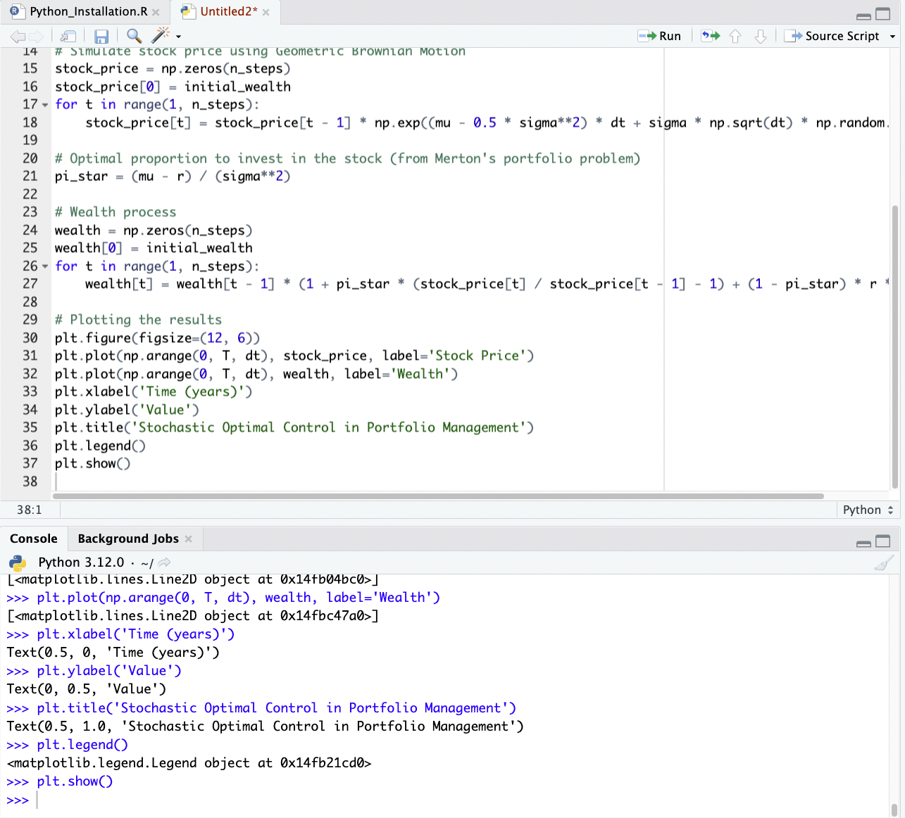
The following Python code sets up and simulates this scenario:

import numpy as np
import matplotlib.pyplot as plt

# Parameters
T = 1.0 # Investment horizon (1 year)
mu = 0.1 # Expected return of the stock
sigma = 0.2 # Volatility of the stock
r = 0.03 # Risk-free rate
initial_wealth = 1000 # Initial wealth
dt = 0.01 # Time step
n_steps = int(T / dt)
np.random.seed(42)

# Simulate stock price using Geometric Brownian Motion
stock_price = np.zeros(n_steps)
stock_price[0] = initial_wealth
for t in range(1, n_steps):
stock_price[t] = stock_price[t - 1] * np.exp((mu - 0.5 * sigma**2) * dt + sigma * np.sqrt(dt) * np.random.randn())

# Optimal proportion to invest in the stock (from Merton's portfolio problem)
pi_star = (mu - r) / (sigma**2)

# Wealth process
wealth = np.zeros(n_steps)
wealth[0] = initial_wealth
for t in range(1, n_steps):
wealth[t] = wealth[t - 1] * (1 + pi_star * (stock_price[t] / stock_price[t - 1] - 1) + (1 - pi_star) * r * dt)

# Plotting the results
plt.figure(figsize=(12, 6))
plt.plot(np.arange(0, T, dt), stock_price, label='Stock Price')
plt.plot(np.arange(0, T, dt), wealth, label='Wealth')
plt.xlabel('Time (years)')
plt.ylabel('Value')
plt.title('Stochastic Optimal Control in Portfolio Management')
plt.legend()
plt.show()

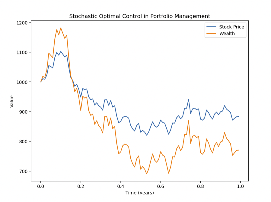
To summarize what we’re doing:

• Simulating the stock price using Geometric Brownian Motion.
• Using Merton’s optimal portfolio rule to determine the fraction of wealth to invest in the stock.
• Calculating the evolution of the trader’s wealth over time.
• Plotting the stock price and wealth process.

In practice, Stochastic Optimal Control problems in finance can be much more complex and may require sophisticated numerical methods and careful consideration of various real-world factors.

Challenges

Model Risk

The reliance on models means that inaccuracies in the model or its parameters can lead to suboptimal decisions.

Computational Complexity

Many problems in Stochastic Optimal Control are computationally intensive, especially in high dimensions.

Overfitting

In machine learning applications, there is a risk of overfitting to historical data, which may not accurately predict future conditions.

Conclusion

Stochastic Optimal Control in finance offers a method for making the best possible financial decisions when facing uncertain and unpredictable market conditions.

For example, it helps in strategically adjusting investment strategies over time, considering the random nature of financial markets to maximize returns or minimize risks.

Its applicability ranges from portfolio management to algorithmic trading, underpinning many of the advanced strategies used in modern financial markets.

Nonetheless, it requires careful consideration of model selection, computational constraints, and the risks associated with stochastic modeling.