Multi-Objective Optimization in Finance, Trading & Markets

Multi-Objective Optimization (MOO) refers to mathematical processes designed to optimize multiple conflicting objectives simultaneously.

Unlike single-objective optimization, which focuses on one goal, MOO addresses scenarios where trade-offs between two or more objectives must be made.

This complexity is common in fields like engineering, finance, economics, policymaking, and logistics.

Key Takeaways – Multi-Objective Optimization

• Balanced Goal Achievement
  • Multi-Objective Optimization (MOO) in finance enables simultaneous pursuit of various goals, like maximizing returns and minimizing risk.
  • Helps lead to well-balanced investment strategies.
• Advanced Algorithm Usage
  • Use algorithms, like genetic algorithms and Pareto optimization, to efficiently navigate trade-offs between conflicting financial objectives.
• Data-Based Decision Making
  • MOO integrates vast financial data sets.
  • Enhances decision-making accuracy in trading and market analysis by considering multiple performance metrics.
• Coding Example
  • We do a type of multi-objective optimization (optimizing for mean, variance, kurtosis, and skew) in a certain portfolio below.

Fundamental Concepts

Objectives and Trade-offs

In MOO, objectives represent the different goals to be achieved.

These objectives often conflict, so improving one may deteriorate another.

The central challenge is finding a balance or trade-off among these competing objectives.

Pareto Optimality

A key concept in MOO is Pareto Optimality.

A solution is Pareto optimal if no objective can be improved without worsening at least one other objective.

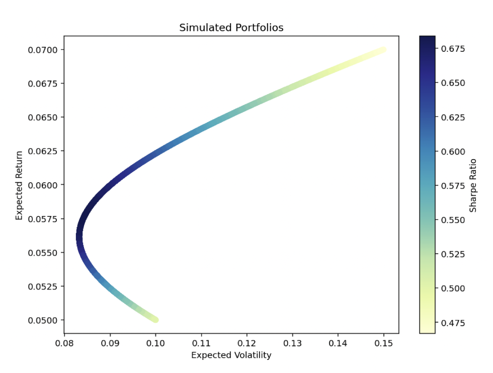
The set of all Pareto optimal solutions forms the Pareto front, which is a tool in MOO for visualizing trade-offs.

Decision Space and Objective Space

Two spaces define MOO:

• the decision space and
• the objective space

The decision space contains all possible solutions, while the objective space maps these solutions to their corresponding objective values.

The interaction between these spaces is fundamental to understanding MOO.

The efficiency frontier diagram for mean-variance optimization is a type of example (the deepest blue part of the graph represents the most optimal combination of assets):

Methodologies in MOO

Scalarization Techniques

Scalarization involves converting multiple objectives into a single objective, often through weighted sums.

This simplification allows the use of traditional single-objective optimization methods.

But it requires careful weighting to avoid bias towards any objective.

Evolutionary Algorithms

Evolutionary algorithms, like genetic algorithms, are well-suited for MOO due to their ability to explore multiple solutions simultaneously.

These algorithms evolve solutions over generations and ideally converge toward the Pareto front.

Multi-Criteria Decision-Making (Analysis)

Multi-Criteria Decision Analysis (MCDA) tools help in selecting the most suitable solution from the Pareto front, based on stakeholder preferences and priorities.

Applications of Multi-Objective Optimization

Engineering Design

In engineering, MOO helps in designing systems that balance cost, efficiency, and performance.

For example, in automotive design, MOO can optimize for fuel efficiency, safety, and cost.

Financial Portfolio Optimization

In finance, MOO is used to balance risk and return in portfolio management.

This involves finding a portfolio that offers the best trade-off between expected returns and associated risks.

There’s also the concept of higher-moment optimization, such as kurtosis and skewness.

Sustainable Development

MOO is used in sustainable development, where environmental, economic, and social objectives must be balanced.

This includes optimizing resource use while minimizing environmental impact and maximizing social welfare.

Challenges & Future Directions

Computational Complexity

MOO is computationally intensive, especially as the number of objectives increases.

Developing more efficient algorithms is an ongoing research area.

Uncertainty and Robustness

Many real-world problems involve unknowns in data and model parameters.

Enhancing MOO to handle uncertainty and provide robust solutions is a key research focus.

Interdisciplinary Integration

Integrating MOO with other fields, like machine learning and data analytics, offers potential for addressing increasingly complex optimization problems.

Coding Example – Multi-Objective Optimization

Let’s consider optimizing a portfolio based on mean, variance, kurtosis, and skewness based on the following criteria:

• Stocks: +6% forward return, 15% annualized volatility using standard deviation
• Bonds: +4% forward return, 10% annualized volatility using standard deviation
• Commodities: +3% forward return, 15% annualized volatility using standard deviation
• Gold: +3% forward return, 15% annualized volatility using standard deviation

To create a Monte Carlo simulation in Python that optimizes a portfolio for mean, variance, kurtosis, and skewness, considering the given assets with their forward returns and volatilities, we need to follow these steps:

• Generate random portfolio allocations for the given assets.
• Calculate the portfolio’s expected return, variance, kurtosis, and skewness (or just assign assumptions since we’re doing a representative example).
• Iterate over numerous simulations to find the optimal portfolio allocation.

Here is an example Python code to achieve this:

import numpy as np
import pandas as pd
from sklearn.preprocessing import MinMaxScaler

# Asset details
assets = {
"Stocks": {"return": 0.06, "volatility": 0.15, "skewness": 1, "kurtosis": 3},
"Bonds": {"return": 0.04, "volatility": 0.10, "skewness": 1, "kurtosis": 3},
"Commodities": {"return": 0.03, "volatility": 0.15, "skewness": 0, "kurtosis": 1},
"Gold": {"return": 0.03, "volatility": 0.15, "skewness": 1, "kurtosis": 1}
}

num_simulations = 10000
results = np.zeros((4, num_simulations))
weights_record = np.zeros((num_simulations, 4))

for i in range(num_simulations):
# Random allocations
weights = np.random.random(4)
weights /= np.sum(weights)
weights_record[i, :] = weights

# Portfolio metrics
portfolio_return = sum(weights * np.array([assets[a]["return"] for a in assets]))
portfolio_volatility = np.sqrt(sum((weights**2) * np.array([assets[a]["volatility"]**2 for a in assets])))
portfolio_skewness = sum(weights * np.array([assets[a]["skewness"] for a in assets]))
portfolio_kurtosis = sum(weights * np.array([assets[a]["kurtosis"] for a in assets]))

results[:, i] = [portfolio_return, portfolio_volatility, portfolio_skewness, portfolio_kurtosis]

results_frame = pd.DataFrame(results.T, columns=["Return", "Volatility", "Skewness", "Kurtosis"])

# Normalize the results to find the optimal portfolio
scaler = MinMaxScaler()
norm_results = scaler.fit_transform(results_frame)
norm_frame = pd.DataFrame(norm_results, columns=results_frame.columns)

# Optimizing for mean, variance, kurtosis, and skewness
# Higher mean and skewness, lower variance and kurtosis are preferred
optimal_idx = norm_frame['Return'].idxmax() - norm_frame['Volatility'].idxmin() + norm_frame['Skewness'].idxmax() - norm_frame['Kurtosis'].idxmin()

optimal_portfolio = results_frame.iloc[optimal_idx]
optimal_weights = weights_record[optimal_idx]
optimal_weights_df = pd.DataFrame(optimal_weights, index=["Stocks", "Bonds", "Commodities", "Gold"], columns=["Weight"])
optimal_weights_df.T

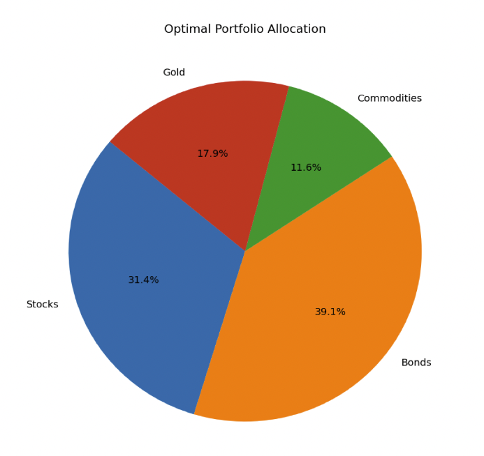
We find that the optimal allocation for this Multi-Objective Optimization (mean, variance, kurtosis, skewness) is:

• Stocks: 31.4%
• Bonds: 39.1%
• Commodities: 11.6%
• Gold: 17.9%

We can also make a diagram:

# Optimal weights 

optimal_weights = [0.314243, 0.390683, 0.116098, 0.178976] 

assets = ["Stocks", "Bonds", "Commodities", "Gold"] 

# Creating a pie chart 

plt.figure(figsize=(8, 8)) 

plt.pie(optimal_weights, labels=assets, autopct='%1.1f%%', startangle=140) 

plt.title("Optimal Portfolio Allocation") 

plt.show()

Note:

• This code assumes assets are uncorrelated.
• All metrics are representative assumptions.
• The optimization logic can be adjusted based on specific investment strategies or preferences.
• Real-world scenarios might require more sophisticated risk management and correlation handling.
• Please be sure to indent this code as appropriate if using it yourself (as shown in the image above).

Conclusion

Multi-Objective Optimization presents a sophisticated approach to handling real-world problems with multiple conflicting objectives.

Its application spans numerous fields, including finance (e.g., portfolio optimization).

Offers a structured way to navigate trade-offs and make informed decisions.

The ongoing evolution of MOO methodologies and their integration with other advanced technologies promises even greater capabilities in solving complex optimization challenges.