Assessing the Value of Control in a Firm


The value of control in a firm represents the level of premium that might be expected to be paid if it were acquired in dollar terms.
When a company is acquired for a majority share, the previous regime is very likely to forfeit its decision-making power, as it’s one of the central objectives in a takeover deal in the first place.
As a consequence, an acquirer can expect to pay a premium that would not apply to a non-controlling takeover where there is no shift in decision-making power.
Whenever there is a stake in control in a mergers and acquisitions deal, there is either a premium applied to the cost of the transaction or a discount involved in transactions lacking any shift in control.
For publicly traded companies involved in large-scale mergers and acquisitions deals, a premium is often paid for taking over the target company beyond its base valuation sum.
The model covered in this article will attempt to assess the value of control in the firm should it be the target of a takeover acquisition. The value is a product of the fact that if a firm is taken over, its acquirer inherently believes that it could run the firm better or merge it with its own operations to cut costs and obtain general efficiency improvements.
Consequently, the value of control in a company is a product of:
a) how much value the acquirer believes would be furnished should it take over and restructure its operations, and
b) the mathematical probability that this operational improvement would occur.
The following spreadsheet (developed by NYU Stern professor Aswath Damodaran and can be found on his website) assesses a company’s control value by the following inputs:
- Beta
- Pre-tax cost of debt
- Tax rate
- Debt to capital ratio
- Revenue
- Operating income (EBIT)
- Pre-tax return on capital
- Reinvestment rate
- Length of the growth period
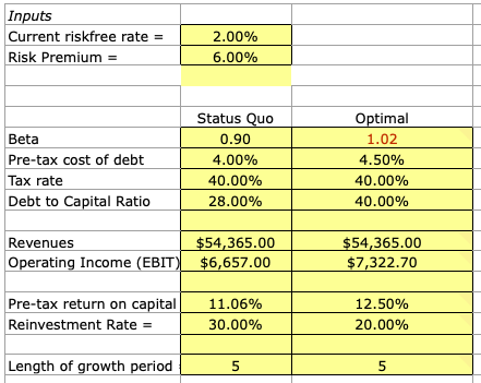 Each input has two values – a status quo value and an optimal value.
The status quo value denotes the company as it is currently, while the optimal value is what the company could become (in a projected or expected sense) under more efficient management.
How are optimal values determined?
One could use target debt ratios (i.e., what does management wish to have as its debt ratio), industry averages for the given set of input criteria, earnings growth targets, and targeted values as a whole.
They are not necessarily objectively derived values, but rather desired and ideally realistic figures.
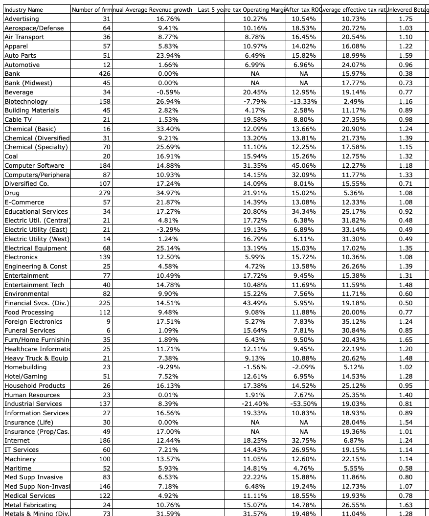
Industry averages are included on a separate sheet within the workbook and have economic data and valuation multiples across all main categories:
 For example, if a firm believes it can cut costs and engage in more efficient operations it will show up in a higher operating income (EBIT) figure.
In the spreadsheet, it is assumed that the optimal figure is 10% higher just as a general measure, although the formula can of course be modified.
But if the acquirer already believes the target firm is operating at optimal capacity – in other words, it has a strong opinion of its management – there is no need to attach a takeover premium, as it only applies to “fixing” scenarios where there is a planned coordinated change in control.
Hints on control value
Below are five things to check for those studying control value in a firm.
1. Check on capital structure to see if a different capital mix can lower the cost of capital (such as using more cheaper debt, or issuing equity if the firm is overleveraged).
2. Check on current pre-tax operating margin and check against industry averages; they may provide clues for potential cost-cutting.
3. Check after-tax return on capital. If it is below the cost of capital, set at least to cost of capital. If it is above the cost of capital, check against industry averages and historical trend line.
4. If return on capital is high, check the reinvestment rate. If it is very low, check to see if there is potential for increase. You can reinvest more or less than you are currently. But consider the consequences for return on capital.
5. If the firm has potential for competitive advantages, see if you can lengthen the growth period (will work only if there are positive excess returns). This is the marginal pre-tax return on capital that you believe that you can earn on new investments. Check the computed values for the after-tax value and how it compares to your cost of capital
How Changes in Inputs Affect the Value of Control
The degree to which changes in given inputs affect the value of control is not an easy question to answer for all inputs given the model inherently relies on “optimal” values.
In some of our models, it’s “higher is better” or “lower is better” given those variables run in a way that scales in one direction only.
However, there are a few variables where this nevertheless does hold true.
EBIT
For instance, operating income as measured by earnings before income and taxes (EBIT) runs on a unidirectional scale.
But this is due to the fact that we also assume that a higher EBIT is better and that we are always underperforming in that respect by 10% to provide an example of a firm that has some work to do to reach optimal levels.
Pre-tax return on capital
Moreover, pre-tax return on capital also runs in one direction.
A higher value is better, as it measures how efficiently the firm is getting a return based on its investment decisions.
The highest value of control (i.e., worst indication of operation) would be situated at 0%, as it would denote the company gets absolutely no return on its capital.
Understandably this is quite bad but (fortunately) difficult to do. On the other hand, if the firm’s pre-tax return on capital is 100% (impossible), the company would have a negative value of control.
This would denote that the company is performing beyond its means.
If we have a negative value of control, it means that we are inaccurate in our assessment of the optimal values to begin with. If perfectly optimal, we would be looking at a value of control value of zero. No premium would be paid as there would be no intent to change the control/decision-making regime in the firm.
Return on capital (ROC) must be greater than the cost of capital for the sake of value creation. If a company, individual, or government is borrowing at a rate higher than the value they’re generating in return, this is value destructive.
Tax rate
The tax rate also represents another sliding scale variable.
The lower the status quo tax rate relative to the optimal tax rate, the lower the value of control.
For instance, if we determine our optimal tax rate is 35%, and the business operates at 40% tax rate based on current operations, the closer it approximates 35%, the lower the value of control will be, representing the better operation.
Reinvestment rate
The reinvestment rate also proceeds in unidirectional fashion. The higher both the status quo and optimal reinvestment rates, the lower the value of control. The reinvestment rate is equal to:
Reinvestment rate = (Capex + Acquisitions + R&D + Other investments) / (EBITDA + R&D + Rent – Taxes)
Capex, acquisitions, investments, and so forth represent a cash outlay.
Consequently, a lower reinvestment rate (i.e., less cash spent) will increase cash flow.
Beta vs. Tax rate and Debt to capital ratio
The beta of the firm’s stock is chiefly a function of its tax rate and debt to capital ratio.
We have discussed how tax rate lowers and raises the value of control depending on the status quo’s proximity to the optimal rate.
However, the debt to capital ratio has a unidirectional impact.
The higher the debt to capital ratio, the higher the optimal beta level.
Beta is a function of the stock’s volatility relative to the market as a whole; 1 is average, >1 is more volatile, <1 is more stable (If zero, then the stock’s returns have no correlation to the returns of the overall market. If negative, the stock has historically moved inversely to the market.)
Given that a higher debt to capital ratio means a more highly leveraged firm, and hence one with more limited financial flexibility, the company’s stock could be expected to be more volatile and have a higher beta as a result.
The higher the beta, the higher the value of control.
A goal for any firm is to possess a lower beta as a mark of greater corporate stability. A lower beta decreases the cost of equity (the discount rate used in the FCFE discounted cash flow model).
A lower cost of equity would thereby increase the present value of all future cash flows and increase the valuation reading of the firm.
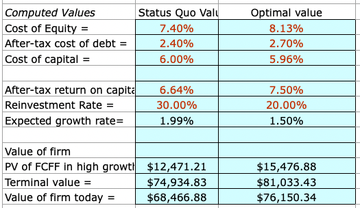
Various calculated values are included at the bottom of the spreadsheet, which feed into the computation of company value.
Length of the growth period
The length of the growth period also has an effect on the value of control.
The longer the growth period, the higher the value of control. This may not seem intuitive at first.
Shouldn’t a better run company have a lower value of control?
It is true that a longer period of high growth will increase cash flows, given longer high growth phases denote greater competitive advantages for the firms undergoing them. When we calculate the value of control we use a simple subtraction:
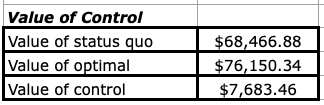
Value of Control = Value of the Firm (optimal) – Value of the Firm (status quo)
If the length of the high growth period goes up, the value of the firm increases due to increased cash flow.
But as a result, the difference in the value of the firms calculated increases based on sheer proportionality.
Example
Let’s say a firm is valued at $10 if all inputs are optimal (perfectly run) and valued at $5 in the status quo period.
The value of control, in this case, would be $10 – $5 = $5.
If the high growth period is extended and this causes the values of the firm to be $14 (if optimal) and $7 (in the status quo), our new value of control would be $14 – $7 = $7.
Even though our cash flows grew proportionally, the difference between the two still grew and therefore our value of control increased as a result.
The value of control and its two components is included at the very bottom of the spreadsheet:
Conclusion
The value of control in a firm involves the act of being able to run the company in a more cost-effective and efficient manner relative to its current degree of operation.
The value of control should be greatest in the most operationally ineffective firms, given there will be the largest disparity between the way it’s run and the way it would most optimally be run.
Often it is a direct consequence of poor management performance, and hence would be deemed “fixable” by decision-makers in the acquiring firm who feel they can do a better firm. This is a common theme is private equity leveraged buyout deals.
Status quo values reflect how the firm is running currently, while optimal values represent an ideal set of circumstances as determined by target debt ratios, industry averages, earnings goals, and other desired attainment of various other financial metrics.
These inputs lead to the formulation of a discounted cash flow calculation at the bottom of the spreadsheet, followed by a terminal value, and company valuation estimation using the FCFF valuation method (i.e., cost of capital used as the discount rate).
The difference between the optimal and status quo FCFF provides the value of control, or the premium associated with enabling a change in executive decision-making power.