The Complete Guide to the FCFF Valuation Model

FCFF is an acronym for “Free Cash Flow for the Firm” or “Free Cash Flow to the Firm” and represents a measure of financial performance related to cash flow.

The popularity of the FCFF valuation model stems from its ability to obtain an accurate valuation of a firm based on a collection of basic inputs.

Why is FCFF important in trading and investing?

FCFF is a form of discounted cash flow (DCF) analysis.

Discounted cash flow analysis is heavily used in business valuation for purposes of real estate development, as an asset valuation method (such as stock valuation), and various corporate finance objectives.

What gives stocks their value is expected cash flow over time – do they have earnings that will earn their shareholders money?

FCFF is a free cash flow model, meaning it’s a way to see how much company cash flow is estimated to be available for distribution among all securities holders (such as a shareholder) without disrupting its operations.

FCFF is equal to operating cash flow minus expenses, taxes, and changes to net working capital (NWC) and investments.

Hence it’s a measure of a company’s profits when all expenses, taxes, and investments are taken into account.

FCFF = Operating cash flow – (Expenses + Taxes + ∆NWC + ∆Investments)

FCFF is one discounted cash flow benchmark among many by which a company’s financial performance is evaluated.

A positive FCFF denotes that the firm has cash remaining after its total costs, whereas a negative value indicates that a firm does not generate enough revenue to cover its total costs and liabilities.

A negative FCFF may represent a red flag to many investors as to why a firm is unable to cover its expenses through its generated revenue.

At its end, one of the central takeaways from the FCFF model is “equity per share,” or the value of a stock in comparison to the equity it generates.

This helps us determine the true worth of the company’s stock in comparison to the price at which it is currently trading and how to find stocks that might be undervalued.

Like any financial model, there are various inputs that must be entered in order to obtain the desired outputs. We will go through each individually.

Inputs

Current Revenues

Revenue is the amount of money that a firm generates through business transactions through the sale of products and services.

Current Capital Invested

The current amount of capital invested in the firm.

An approximate estimate can be determined by the book value of debt plus the book value of common equity.

Current Depreciation

Every firm will suffer some form of depreciation in the value of its assets and is accounted for via depreciation.

Current Capital Expenditures (often abbreviated as Capex)

Capital expenditures represent the amount of money a firm spends on physical, non-consumable assets such as investments into plant, property, and equipment (PP&E), or forms of machines and infrastructure to assist in business development.

Change in Working Capital

This is defined as the change in the number of assets minus the change in the monetary value of current liabilities.

Assets must increase or liabilities must decrease – or some net favorable combination – for net working capital to increase in value.

Value of Current Debt Outstanding

A firm’s amount of current payments owed.

Number of Shares Outstanding

This is the number of shares that a firm currently has circulating.

FCFF: High growth period + Stable growth period

Discounted cash flow is often broken into two parts – a 5-10 year higher-growth period followed by the calculation of a terminal value beyond that.

An FCFF valuation is likewise broken down into two additional components – a high growth period and a stable growth period.

When a firm is just starting out, it may expect to undergo a high growth period as it brings itself up to speed with competitors.

However, for a mature company, growth will tend to be more stable as it’s established itself in its markets and there are fewer opportunities to grow.

This is also seen in growth at the national level. Over the preceding decades, countries like China and Korea have seen explosive growth due to technological and industry-based advancement that was absent previously.

However, a country such as the United States, which has already made those advancements, will experience more stable, incremental growth.

We’ll go through each period individually:

High Growth Period

Revenue Growth Rate for the Next 5 Years

The growth rate input is typically the first thing that’s considered.

Selecting five years is somewhat arbitrary, but is typically the standard used in many FCFF models, as it’s difficult for a firm to maintain high growth beyond about a five-year period.

Others might consider a high-growth period going for ten or even fifteen years.

Operating Expenses as % of Revenue in Fifth Year

Operating expenses should always be lower than revenue to sustain a profitable business.

The figure comes to 70%-75% for many firms. Depreciation is included in this figure and is equal to 1 – (Before Tax Operating Margin).

Growth Rate in Capital Expenditures & Depreciation

This represents the aggregate sum of money invested in physical capital (e.g., plant, property, and equipment) and the depreciation rate associated with any assets specific to the firm.

Debt as a % to Use for Financial Investments

Written another way, of all debt associated with the firm, what percentage of it is in use for financial investments?

Normally this figure is low. For some firms, it might very well be zero.

Working Capital as a % of Revenues

Working capital, as aforementioned, represents assets minus liabilities.

Here it would be expressed as a percentage in terms of gross revenue.

Tax Rate on Corporate Income

This is simply the rate at which the firm would be taxed by the central government.

Beta for Calculating Cost of Equity

Beta determines a firm’s share price sensitivity against market movement in general. A beta of one is average. Its shares react to market movement at the average rate.

• Betas above one are less stable and see more volatile, over-reactive movement.
• Betas below one demonstrate stocks that are more stable in nature.
• A negative beta would denote a share price that moves opposite the general direction of the market.

The stereotypical example of a negative-beta stock would be that of a gold-mining business.

Investors will often tend to invest in gold when the stock market isn’t producing positive returns.

Hence a gold-mining company might see its stock rise in negative market conditions and yield a negative beta.

Companies undergoing a high-growth period regularly see betas surpassing one. In stable periods, beta is more likely to approximate one, or market average.

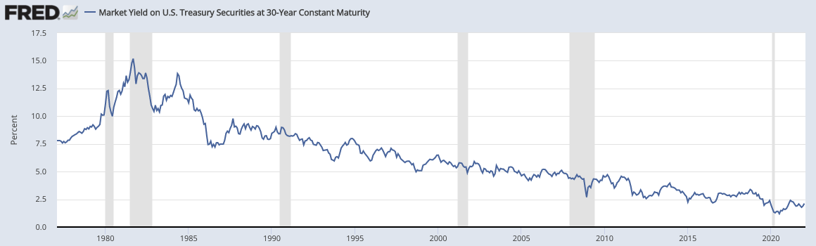
Current Long-Term Bond Rate

Long-term bond yields in the US have been in a near-steady state of decline since the early 1980s returning.

The long-term bond rate is important as it figures into the calculation of cost of equity.

The long-term bond rate gives us the risk-free return in the market.

Knowing this input, we can easily feed it into a cost of equity calculation, which is the risk-free return in the market added to the product of beta and the risk premium of market assets versus risk-free assets:

• • E = Rf + ß(Rm – Rf)

Where:

E = Expected rate of return for that security
Rf = Risk free rate of return in the market (i.e., government bond yield)
Rm = Historical return of the stock market (can be narrowed by sector and time range)
ß = Market risk sensitivity (1=average; <1=more stable; >1=more volatile)

Market Risk Premium

Equal to the historical return of the stock market against the risk-free rate of return given by long-term government bond yield.

Represented by Rm-Rf in the above equation.

Cost of Borrowing

The interest rate at which the firm could obtain a loan.

The stable growth period includes fewer factors and many overlap from the high-growth period.

Stable Growth Period

Revenue Growth Rate

In the high-growth period, we can see revenue growth of 25% or better depending on many factors. A more mature company in a mature industry with several competitors will see slower growth somewhere in the single-digits normally.

A 5%-6% growth represents a stable level of growth that will normally keep a company plugging along. Once a company enters the stable growth phase it becomes more and more difficult to improve.

Operating Expenses as % of Revenues

Operating expenses are typically a bit higher for firms during a stable growth period, as a percentage of revenue.

But ideally they will still be less of a percentage for the company to maintain long-term solvency.

Capital Expenditures as a % of Depreciation

This can be calculated in one of three ways.

1. Assume net capital expenditures are equal to zero.

This is the most common way and renders capital expenditures as equal to 100% of depreciation.

2. Assume the capital expenditures / depreciation ratio is equal to the industry average

3. As a proportion of (Growth rate in operating income) / (Expected return on capital).

This provides a value known as net capital expenditures. This number could then be divided by depreciation to determine the ratio needed.

Debt as a % for Financial Investments

The percent of debt that comes in the form of financial investments.

Interest Rate of Debt

Debt is charged a premium via accumulated interest, such that the lender can earn a profit by offering to lend money in the first place.

This would be the aggregate figure for all forms of debt.

Beta for Calculating Cost of Equity

Beta is more likely to be nearer to the market average in a stable growth period, reflecting greater stability in the company.

Bloomberg is commonly used to estimate betas and what might be the most appropriate to use for a cost of equity calculation.

Outputs

After our inputs are put into place, we can obtain outputs of interest, such as estimated cash flows, cost of equity and capital, and approximate valuation of the firm. We will go over each of their sub-components below.

Growth in Revenue

The high-growth period is automatically assumed within the model to be of five years, and projects out to ten years in the future.

Years 1-5 of the model are considered the “high-growth years,” years 5-9 represent a transition period into the stable growth period (lower successive growth each year), with year 10 estimating what cash flow should look like during the stable growth period.

The calculations are based on assumptions of both how long the high-growth period lasts and how long the transition takes into the stable growth period. For convenience sake, the spreadsheet assumes five years each.

Growth in Depreciation

The growth in depreciation follows the same pattern as growth in revenue.

The calculation is the exact same in our spreadsheet, but uses “Growth Rate in Capital Expenditures and Depreciation” instead of “Revenue Growth Rate.”

It is constant for the first five years, then undergoes a five-year transition into the stabilization period.

Revenues

We can calculate revenues by taking revenue from the base period (i.e., whatever we are designating as our starting point) and multiplying that by [1 + (Growth in Revenue)] to determine revenue in the next period.

For example, if our base period revenue was $200,000 per year and our annual revenue growth rate is 25%, then our revenue the next year projects to be: $200,000 * (1 + 0.25) = $250,000

Operating Expenses

Operating expenses are calculated by taking operating expenses as a percentage of revenues (an input) and multiplying by revenues from the same time period.

EBIT

Acronym for Earnings Before Interest and Taxes. It is equal to Revenues minus Operating Expenses.

EBIT (1-t)

This value is the same as Revenues minus Operating Expenses but with taxes taken out.

The “1-t” articulates what we need to multiply by in order to determine the value, which is 1 – (Tax Rate).

For example, if the firm is taxed at a rate of 21%, that means we have 79% (1 – Taxes) of our earnings remaining. If our profit is $200,000, after taxes we have $158,000 remaining.

FCFF

In order to calculate the model’s namesake, the free cash flow to the firm, we must take EBIT (1-t), add depreciation, subtract capital expenditures, and subtract change in working capital.

These are all values, of course, we derive from inputs into our model.

Depreciation is depreciation from the base period multiplied by [1 + (Growth in Depreciation)].

Capital Expenditures is capex from the base period multiplied by [1 + (Growth Rate in Capital Expenditure and Depreciation)].

Change in Working Capital is equal to Working Capital as a Percentage of Revenues multiplied by the difference between current revenues and revenues in the previous period.

So for instance, if our working capital as a percent of revenues was 10%, this year we have a revenue of $250,000 and in the previous year $200,000, our change in working capital would be assessed as:

• • 0.10 * ($250,000 – $200,000) = $5,000

Terminal Value

Theoretically, we could calculate discounted cash flows ad infinitum.

But to obtain some sort of closure on what our cash flows are telling us, we compute what’s called a terminal value.

It is the present value of all future cash flows at a future point in time when we expect cash flows to follow a stable pattern of growth.

Forecasting beyond a certain point is impractical given industry and macroeconomic conditions become consistently more difficult to predict.

Hence we can cap off our discounted cash flow by a terminal value calculated via a type of perpetuity growth calculation (i.e., the Gordon growth model).

Since the model we’ve set up consists of ten years, five in a period of high growth and five in a period transitioning into stable growth, we calculate the terminal value after ten years.

We do this by taking the final FCFF value in year 10 (i.e., last year of the model), multiply by [1+ (Revenue Growth Rate of the Stable Period)] and subsequently divide by the (Cost of Capital in the Final Year – Revenue Growth Rate of the Stable Period).

This gives the FCFF valuation of a company based on the assumption that it will resume its cash flow at a rate of stable growth throughout its life.

Cost of Capital and Equity

For the cost of capital and equity we calculate seven main components:

Cost of Equity

Represents the return a company pays its shareholders for the risk undertaken to invest in their stock.

It is essentially the minimum rate of return that investors demand in order to determine that the company is worth investing into.

In terms of how it’s calculated when it comes to academic corporate finance, it is equal to:

(Beta for Calculating Cost of Equity) * (Market Risk Premium) + (Current Long-Term Bond Rate)

Proportion of Equity

Defined as: 1 – (Debt as a Percentage to Use for Financial Investments)

After-tax Cost of Debt

Defined as the (Cost of Borrowing Money) * (1 – Tax Rate). This is usually a single-digit percentage. If the interest rate at which a firm could borrow money is 10% and the tax rate is 36%, the After-tax Cost of Debt would be:

• • 0.10 * (1 – 0.36) = 0.064 = 6.4%

Proportion of Debt

This is simply 1 – (Proportion of Equity).

The proportion of debt and proportion of equity will always naturally add up to 1, or 100%.

Some securities are hybrids of the two, like preferred stock and convertible bonds.

Cost of Capital

The cost of capital is defined by a function consisting of the previous four components.

• • Cost of Capital = (Cost of Equity) * (Proportion of Equity) + (After-tax Cost of Debt) * (Proportion of Debt)

Cumulative WACC

WACC (the weighted average cost of capital) can be defined as the rate at which a firm measures the cost of financing capital for an internal project.

A lower WACC is generally considered a good thing.

The lower a company’s WACC, the easier it will be to fund new projects, as the metric allows the firm to calculate how much it would cost to finance it.

Mathematically it can be defined as:

• • (Cumulative WACC of preceding period) * (1 + Cost of Capital)

Present Value

WACC also allows us to calculate the present value of the firm within a given year. We do this by dividing FCFF by Cumulative WACC.

In our present valuation for the final year, we will need to add FCFF to our Terminal Value and then divide that figure by Cumulative WACC.

This is extremely important to do, as a failure to do so will give a very inaccurate estimated firm valuation later on.

If we don’t do this, then we aren’t obtaining the aggregate Present Value over the life of the company; we are merely doing it for ten years.

Firm Valuation

Finally, we can delve into deriving the estimated value of the firm.

We will use our outputs obtained from the previous section to determine the value of the firm, subtract any outstanding debt to determine the value of equity.

Then, we’ll divide the value of equity by the number of shares in circulation to obtain a projected valuation of the company’s stock.

Value of the Firm

This is equal to the sum of our present value computations derived in the previous calculation row. The =SUM function in Excel will do this easily by providing the range of cells needed to add together.

Value of Debt

To derive the value of equity, we need to subtract the value of debt from the value of the firm to obtain an accurate estimation.

Value of Equity

The total estimated value of a firm’s shares in circulation. Equal to (Value of the Firm) – (Value of Debt).

Value of Equity per Share

This estimates the true value of a firm’s stock, to denote if it’s undervalued, overvalued, or fairly valued relative to the price at which it’s currently trading.

Equal to: (Value of Equity) / (Number of Share Outstanding)

Value of the Firm by Year

This assesses the value of a firm for each year reported in the model.

For the initial year, this is the Value of the Firm.

For each subsequent year, this is the sum of the present values calculated earlier from the year being calculated onward multiplied by Cumulative WACC.

For instance, if we are attempting to assess the value of the firm from the second year, we would only sum the present values from the second year onward.

For assessing the value of the firm in the third year, we only sum the present values from the third year onward, and so forth.

And of course, multiply that sum by Cumulative WACC as the ever-important financial barometer of how easily a company can finance a project.

Value of Debt

This is to obtain the value of debt within a given year.

This is defined as the proportion of debt (i.e., a percentage) within the given year multiplied by the value of the firm within that same year.

If we wanted to calculate the value of debt of a firm, we would do: (Proportion of Debt %) * (Value of the Firm ($))

Conclusion: FCFF Valuation Model

In the end, FCFF is designed to work as another discounted cash flow model that can accurately assess the value of a company from a set of given inputs.

For a company, it can shed light on ways of improving cash flow based on manipulation of the given inputs and is one model available that can calculate cash flow based on the accounting information at hand.

The FCFF model is valuable to traders and investors as it determines helps determine how to calculate equity value, or what the “true” share price of a company should be.

Is this company undervalued, overvalued, or fairly valued?

If undervalued, we might have a bargain and recommend adding it to a personal or company portfolio.

Then again, when attempting to value companies we must always keep in mind that we are making many assumptions regarding its cash flow.

We can nail down some inputs based on accessible data. However, at the same time, we must leave some buffer room in our valuation in order to recognize that the assumptions we’re making might be overestimating or underestimating the quality of this company and its stock.

For instance, if based on our FCFF calculation we determine that the fair share price of this company is $45.00 and it’s currently trading at $50.00, we might think this is a good deal.

But is $5.00 enough of a cushion? Maybe the model is off in its true valuation by 6% against us, leaving only a $2.00 undervaluation.

Consequently, we need to be more conservative in our approach. Moreover, there are numerous valuation means on how to value stocks and how to find stocks that are undervalued relative to their current trading price.

We can value a company via other discounted cash flow models as well, including FCFE, dividend discount models, enterprise value based multiplier models, and asset-based models, as well.

This can help triangulate the value of a company or stock by various methods.