The Complete Guide to the FCFE Company Valuation Method

Free cash flow to equity (FCFE) is another discounted cash flow model of how to calculate company valuation. It is a measure of how much cash can be provided to equity shareholders of a firm when all expenses and debts are accounted for (i.e., levered cash flow). In a way, it is similar to dividends.

Actual dividends are what is paid to shareholders; potential dividends are represented through FCFE. The FCFE model is typically used as part of a discounted cash flow (DCF) or leveraged buyout (LBO) valuation.

By itself FCFE can be mathematically calculated as:

FCFE = Net Income + Depreciation & Amorization + Net Borrowing – (∆Working Capital + Capital Expenditures)

Where:

• Net Income = Income – Cost of goods sold – Expenses – Taxes
• Depreciation & Amortization = Decline in value over time
• Net Borrowing = New debts – Debt repayments
• ∆Working Capital = Current assets – Current Liabilities
• Capital Expenditures = Expenditures used to upgrade or acquire fixed assets, like plant, property and equipment (PP&E)

FCFE differs from FCFF (free cash flow to the firm) in that FCFE relates to the cash available to the firm’s shareholders only.

FCFF represents the cash that can be distributed to all stakeholders – shareholders, preferred shareholders, bondholders, and any additional person with a holding claim to the company.

Mathematically the relation between FCFE and FCFF can be stated as follows:

FCFE = FCFF + Net Borrowing – Interest (1-t)

Where:

• FCFF = cash available to all claimholders associated with the firm
• Net Borrowing = New debts – Debt repayments
• Interest (1-t) = Interest multiplied by (1 – tax rate) (i.e., interest expense)

The FCFE (Free cash flow to equity) Model

Those using FCFE commonly use a three-stage discount model, as it’s the most involved of the three basic forms (the others being a one-stage and two-stage).

A one-stage model is specifically for firms undergoing a period of stable growth.

A two-stage model is most appropriate for firms undergoing moderate growth and is also a very common form that is used for firm valuation.

A three-stage pertains to businesses undergoing high growth with the implicit understanding that they are likely new and will eventually slow to a stable period of growth over the long run.

A three-stage is normally most appropriate for a startup.

One of the more common FCFE templates online was developed by Aswath Damodaran from NYU Stern (link).

You can build many of these from scratch if you wish, although it isn’t essential. It is, however, important that if you do use a spreadsheet to understand each cell and its purpose to completely grasp a financial model.

The model makes the following assumptions:

1. Because we are using a three-stage FCFE discount model, we are assuming the firm is in a period of high growth.

2. The high-growth phase runs for a certain period of time that has to be specified within the spreadsheet.

3. During the transition from high growth to stable growth, the decrease in growth rate will occur in a linear fashion.

4. Capital spending and depreciation rate change consistently with the growth rate.

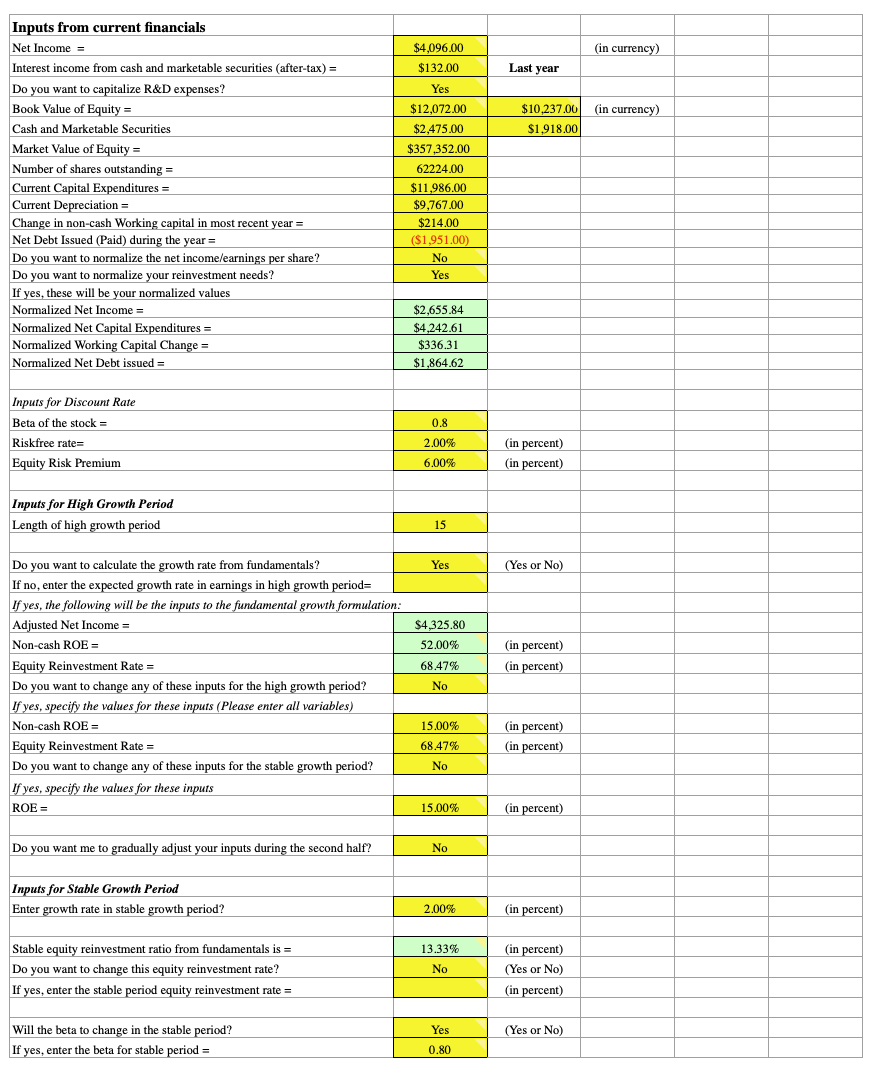
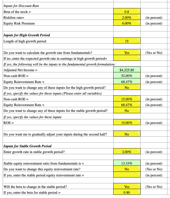
The user will be expected to input the following related to the growth phase(s): length of each growth period, growth rate used to define the high growth and stable growth periods, and capital spending, depreciation, working capital, and costs of equity within each phase.

Much of the data involved will be findable from sources such as Bloomberg, Morningstar Direct, and various free avenues on the internet.

These include the basic, general inputs of the model of:

• earnings per share
• current dividends per share
• capital spending per share
• depreciation per share
• revenue per share
• working capital per share, and
• change in working capital per share

The cost of equity of the firm can also be entered if available.

If not, then inputs will need to be made regarding the beta of the stock, the risk-free rate, and risk premium – i.e., the three variables that go into the cost of equity equation (i.e., COE = Risk-free rate + ß * Risk premium).

The risk-free rate is essentially the treasury bond yield as its closest approximation. (The discrepancy between a true risk-free investment and the treasury bond yield is the probability of that country defaulting on its debts – essentially zero for a country such as the US, which can always at least pay in nominal terms.)

The risk premium pertains to the difference of risk difference between market assets and risk-free assets. Determining this is a matter of estimation.

Typically, the value taken as the risk premium separating stocks and risk-free bonds has been found to vary between about 3 to 7 percent.

For example, if a 10-year bond yields 2 percent and stocks are trading at a forward P/E of 20x (inverse is the yield, or 5 percent), the the risk premium is taken as 3 percent.

The beta of a stock is a measure of how volatile it is relative to the market. A beta of 1 is considered the market average.

Betas above one represent more volatile stocks (such as those from companies undergoing a high-growth period), while betas below one represent more stable stocks (such as those from companies undergoing stable growth).

Beta is modifiable between the high-growth and stable-growth periods in the spreadsheet.

Generally, as companies survive longer their financial performance becomes steadier and their beta drops to reflect this greater predictability.

Cost of equity components vs. Stock price

There are a few main notable influences on stock price from the variables in a cost of equity equation:

1. A higher risk-free rate decreases stock price.

This makes logical sense in terms of what we see in terms of actual investment behavior.

As the stock market falters, investors typically head more toward bonds, especially if the drop is deflationary.

When the stock market is in more robust shape, bonds are less popular.

2. A higher risk premium decreases the stock price.

Generally, when there is increased risk regarding a certain asset, it will decrease its inherent value.

For each incremental increase in risk premium, there will be an exponential decrease in the stock’s value.

For instance, the stock’s value will decrease more from a risk premium jump from 5% to 6% than from 4% to 5%.

3. A higher beta decreases the stock price.

Following the same reasoning as a higher risk premium decreasing a stock price, a more volatile, higher beta stock will also decrease the stock price.

4. A higher cost of equity will also decrease stock price.

Since the cost of equity entails the rate of return required to incentivize investors to buy shares of that company’s stock, a higher cost of equity would in turn make the stock less valuable.

There are a few choices that need to be made in the spreadsheet:

One regards the cost of equity.

It can either be entered manually, or the spreadsheet can do the calculation via risk-free rate, beta, and risk premium inputs.

The spreadsheet will ask you if you wish to calculate the growth rate of the firm from fundamental values respective of both the high-growth and stable growth period – i.e., return on capital (ROC), D/E (book value of debt/book value of equity), interest rate, and retention (1 – dividends per share/earnings per share). Select no if the growth rate of the firm is already known.

Otherwise, type yes.

The spreadsheet will ask if capital spending is offset by depreciation in the stable period. If the answer is yes, then you will enter the return on equity that your firm will have in perpetuity.

If the answer is no, then you will enter capital expenditures as a percent of depreciation.

Next, you will be asked a question regarding whether you want to calculate your investment rate from fundamentals? If we are assuming perpetual growth – i.e., high-growth eventually leading to stable growth that in turn lasts for the life of the company – then the answer should be no.

You will need to ensure that capital expenditures are higher than depreciation in your terminal year.

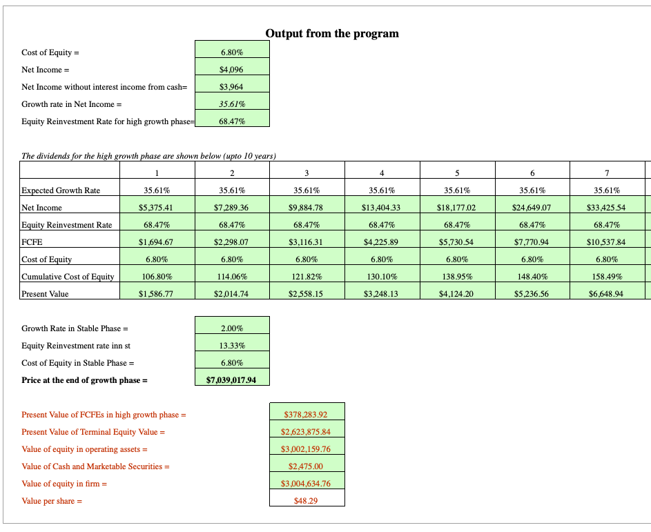
Calculating Outputs

Since this model is inherently about FCFE, many of our inputs will feed into the FCFE calculation, with its terminal value going on to determine the fair value of the firm’s share price. For purposes of this spreadsheet, FCFE is calculated through one interpretation of the definition shared earlier:

FCFE = Earnings per share – (Capital Expenditures – Depreciation) * (1 – Proportion of debt from Capital Spending) – (∆Working Capital) * (1 – Proportion of debt from Working Capital)

In the transition period…

• growth rate
• cumulated growth
• beta
• cost of equity, and
• the present value of FCFE during the transition phase…

…all change in linear fashion ordering to any aforementioned trade inputs.

However…

• earnings per share
• (capital expenditures – depreciation) * (1 – Proportion of debt from capital spending), and
• (∆working capital) * (1- Proportion of debt from working capital), and
• FCFE…

…all increase exponentially due to the nature of their calculations.

The terminal value calculation of:

• earnings per share
• (capital expenditures – depreciation) * (1 – proportion of debt from capital spending), and
• (∆working capital) * (1- proportion of debt from working capital)…

…are based off multiplying the values from when the period of stable growth begins by (1 + growth rate in revenues).

The growth rate in revenues is an estimation usually based on the industry average.

The terminal value of FCFE is determined by adding those three terminal values together.

Determining Stock Price

There are two main calculations to be made – the first being future stock price estimation at the end of the stable growth period.

In other words, this is the ultimate value the stock can realistically expect in today’s dollars – based on future outlook and under our current inputs.

The second regards the present value of the stock price.

In other words, how might this stock be valued relative to its currently traded price?

From our inputs, we will be able to ascertain both.

For the future price, we calculate the equivalent of a terminal equity calculation.

This is just like in any discounted cash flow model that’s popular in investing, banking, and other financial disciplines.

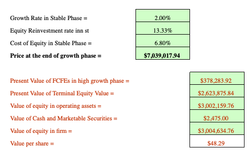
We look toward projected growth rate once the firm is situated within a stable growth phase, FCFE in the terminal year (i.e., FCFE once the stable period begins), and cost of equity in the stable growth phase.

Mathematically, the relationship can be expressed as:

Price = FCFE in terminal year / (Cost of equity in stable phase – Growth rate in stable phase)

It is similar in method regarding how to calculate equity value.

For the current valuation of the stock, we need the following:

• Present value of FCFE in the high-growth phase
• Present value of FCFE in the transition period from high growth to stable growth and
• present value of the terminal price just calculated

The present value of FCFE has already been calculated from inputs earlier in our spreadsheet.

We simply sum the cells relevant to each growth phase.

The calculation for the present value of our terminal price is more involved. But in short, it is equal to the terminal price just calculated divided by the sum of (1 + Cost of equity) for all high-growth and transition phase years. Mathematically:

Terminal price / ∑ (1 + Cost of equity)

With this, we’ve derived the final price of the stock.

In the example data that come entered into the spreadsheet by default (using the Damodaran spreadsheet linked above), the stock is presently valued at $48.29.

If the stock is trading at $50 in the market, it could be considered about fairly valued or slightly overvalued and may not be a recommended buy based on valuation reasons.

If the stock is currently trading at $45, then we might consider the stock undervalued by 10 percent.

But on the same token, we have to be careful, given that assumptions are built into our model, and 10 percent might not be much in the way of buffer room to give outright confidence in our determination that this stock could be a bargain.

In the end, all that’s known is baked into the price. So to add value to a market (earn in excess of a representative index) – i.e., generate alpha – you have to have an out-of-consensus view and do better than the average market participant.

Conclusion

The FCFE model provides insight into the amount of dividends that a firm can afford to pay.

The model is essentially shareholder-centric by accounting for how much cash can be paid to stockholders only.

This is different from the FCFF model, which includes the amount of cash that can be distributed to all stakeholders – i.e., bondholders, preferred shareholders (if applicable), warrant holders (if applicable), and so on.

FCFE is equal to FCFF plus net borrowing minus after-tax interest expense.

When a firm is entirely financed by equity FCFE and FCFF are equal to each other.

For all discounted cash flow models, the determination of cash flows present value comes in the form of:

PV of cash flow = CF(t) / (1 +k)

• CF(t) = the cash flow in a particular period, t
• k = discount rate specific to a particular asset

Some may view FCFE as superior to FCFF for determining share value by using the cost of equity as its discount rate when calculating the present cash flow value rather than the weighted average cost of capital (WACC).

FCFE uses the cost of equity relative to the firm rather than a market value of equity, such as WACC.

In any case, both methods are employed because of their abilities to generate robust valuation estimates.

When employed in conjunction, one can better help inform the other in terms of final equity value estimates, rather than one used exclusively.