The Complete Guide to the Dividend Discount Model (DDM)


The dividend discount model (DDM) is a method of valuing a company’s stock based on discounting the sum of all future dividends in terms of present value. In this case, we will be using a two-stage dividend discount model.
Two-stage models tend to be the most common when evaluating firms.
They entail valuing the amount of equity in a firm that undergoes two stages of growth – a high-growth phase and a stable-growth phase where the company proceeds at a moderate rate of growth.
For frame of reference, you will be right at the intersection of these two periods when making your valuation of the firm. That is, right at the end of the high-growth phase or beginning of the stable-growth phase.
The assumptions inherent in this model dictate that the firm will be expected to grow at a higher rate at the beginning of the period, fall linearly at the end of it, and then proceed at a stable rate of growth for the second period.
Moreover, it is implicitly assumed that the dividend payout rate will be linearly congruent with the growth rate.
This two-stage DDM was developed by NYU Stern Professor Aswath Damodaran and can be found under the label ‘ddm2st.xls‘ (download link) on his website.
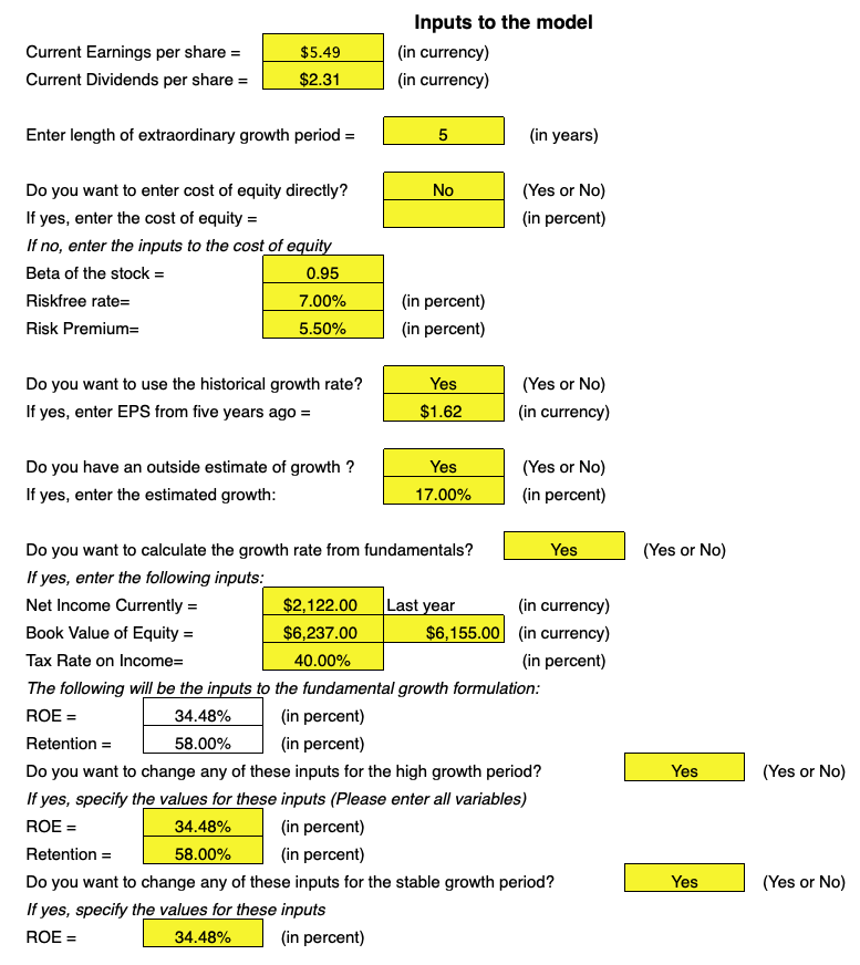
In order to derive the value of equity within the firm and its resultant projected fair value share price, the following inputs need to be defined:
1. Earnings Per Share (both current EPS and from a specified point in the past)
2. Current Dividends Per Share
3. Length of High Growth Period
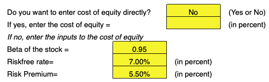
4. Cost of Equity (or derived from the inputs of the company stock’s beta, risk-free rate, and risk premium)
5. Estimated Growth in Earnings during Stable Growth Period
6. Growth Rate (or from the fundamentals of current net income, book value of equity, tax rate on income)
7. Historical Growth Rate
8. Outside Prediction of Growth
 All this information shouldn’t be too difficult to procure through a platform like Bloomberg, Morningstar Direct, Reuters, or even many of the open-source tools available online.
Earnings per share is measured by:
(Net Income – Preferred Stock Dividends) / (Outstanding Shares).
Dividends per share is measured by:
(Total Dividends Paid Out in Past Year) / (Outstandings Shares).
Note that it is very important to input the components of the cost of equity correctly.
The price of a stock with respect to modeling valuation is hypersensitive to inputs of beta, risk-free rate, and risk premium to the point where simple deviations from the actual values can produce substantially flawed estimations of a firm’s equity and consequent stock value.
Even being off by a mere 1% with respect to the risk premium can throw off a stock’s estimated value by nearly 100%.
Moreover, if we are off in our beta estimate by 0.1 (and we shouldn’t be as this info will be readily accessible), it can change our stock price valuation by nearly 100%, as well.
Even if the error input caused linear distortion in our outputs, it would muddy our analysis. But exponential distortion on a 100:1 scale would invalidate the entire valuation. So needless to say, it is essential to have our cost of equity inputs as correct as possible.
 And to mirror what was stated in The Complete Guide to the FCFE Company Valuation Method, a higher cost of equity will decrease a stock price.
The cost of equity is simply the rate of return that must be produced by the company to incentivize investors to purchase the stock.
For instance, if a company has a cost of equity of 10%, then investors will expect this company’s stock to generate at least a 10% annual return to consider investing in it.
The higher the cost of equity, the riskier the stock, and hence the lower its intrinsic value.
To estimate growth rate, if it is not readily available on its own, a few inputs will need to be entered. Current net income, book value of equity, and tax rate on income should be readily available through online databases.
From these inputs, the return on equity (ROE) can be calculated, which is equal to:
Current Net Income / Book Value of Equity in the previous year
Our retention percent is simply:
1 – (Current Dividends Per Share) / (Current Earnings Per Share)
A higher ROE will have the effect of increasing stock price, while a higher retention rate will also have the effect of increasing stock price.
Earnings per share will need to exceed dividends per share in order to have a positive retention rate.
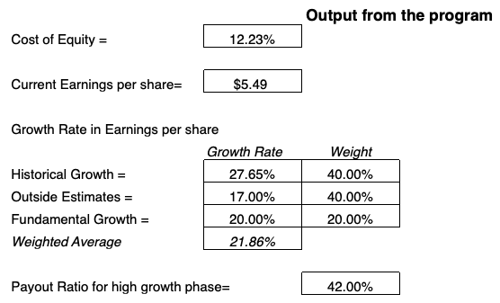
The payout ratio for the high growth period will be 1 – (Retention rate).
A higher current dividends per share price will decrease projected stock price value.
Deriving Outputs from the Model
To determine the projected price of the share at the end of the stable growth phase (i.e., long-term outlook), it will be a function of:
- the current earnings per share (EPS)
- a weighted average of growth factors (historical growth, outside growth estimates, and fundamental growth)
- the length of the high growth period
- the growth rate
- payout ratio, and
- cost of equity in the stable growth period
 The formula follows as:
Terminal Value of the Stock = (Current EPS) * (1 + Weighted Average of Growth Factors) ^ (Length of High Growth Period in Years) * (Payout Ratio in Stable Phase) / (Cost of Equity in Stable Phase – Growth Rate in Stable Phase)
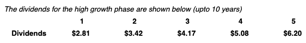
We can also obtain dividend values for the high growth period leading up to the stable growth period.
For the end of the first year, our projected dividend would be equal to:
(Current EPS) * (1 + Weighted Average of Growth Factors) * (Payout Ratio in High Growth Phase)
For each subsequent year during the high growth phase, it will be based on the previous year’s dividends multiplied by one plus the weighted average of growth factors:
(Previous Year’s Dividends) * (1 + Weighted Average of Growth Factors)
In addition to the cost of equity, the value of a firm’s stock price is hypersensitive to its rate of growth during the stable period.
For each successive 1% increase in growth rate, there is an exponential increase in its effect on stock price.
For example, an increase in growth rate during the stable period from 5% to 6% can increase current stock price valuation by 25%. Going from 6% to 7%, by 37%. And from 7% to 8%, by 69%.
This is non-linear increase is the result of the mathematical framework on which the DDM model is built, known as the Gordon Growth Model:
P = D / (r – g)
Where:
P = Price of stock
D = Value of next year’s dividends
r = Cost of equity in the stable growth phase
g = Growth rate in stable phase
We know that once the size of the denominator shrinks, the estimated worth of the stock will increase exponentially.
For a fuller articulation of a Monte Carlo simulation that was performed on the DDM to see how change in the cost of equity and growth rate affected stock price, please see: Estimating Stock Price with Linear Regression
To determine stock price, we still need to determine two more items – the present value of dividends in the high growth phase and present value of the terminal price of the stock.
The present value of dividends in the high growth phase is one of the more intricate calculations in the DDM model, but still follows the basic structure of the Gordon Growth Model. It is equal to:
PV of Dividends in High Growth Phase = Current EPS * Payout Ratio for High Growth Phase * (1 + Weighted Average of Growth Rates) * (1 – ((1 + Weighted Average of Growth Rates)) ^ (Length of High Growth Period) / (1 + Cost of Equity) ^ (Length of High Growth Period) / (Cost of Equity – Weighted Average of Growth Rates)
Next we have to calculate the present value of the terminal price of the stock. This is simply the current stock price minus the value of dividends in the high growth phase.
It’s equal to:
PV of Terminal Stock Price = Price at the End of Stable Growth Phase / (1 + Cost of Equity) ^ (Length of High Growth Period)
The current value of the stock (basically the grand finale output) is the sum of these two components:
Current Value of the Stock = PV of Dividends in High Growth Phase + PV of Terminal Stock Price
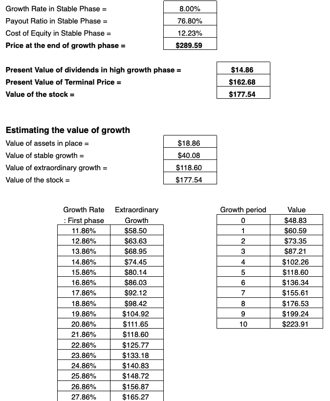 We can also go ahead and calculate estimates of the value of growth in terms of three components: Value of Assets in Place, Value of Stable Growth, and Value of High Growth.
We calculate the value of assets in place by:
Value of Assets in Place = Dividends Per Share / Cost of Equity in Stable Growth Phase
Value of stable growth:
Value of Stable Growth = Dividends Per Share * (1 + Growth Rate in Stable Growth Phase) / (Cost of Equity in Stable Phase – Growth Rate in Stable Phase) – Value of Assets in Place
The value of high growth is equivalent to the current value of the stock just calculated and subtracting the value of assets in place and value of stable growth:
Value of High Growth = Current Value of the Stock – (Value of Assets in Place + Value of Stable Growth)
If we sum these three values of growth, we will also obtain the current valuation estimate of the current stock.
Additional Items
Projected dividends for each year of the high growth period are calculated:
 Moreover, at the very bottom of this spreadsheet, there are a couple features available to allow analysts to see how the value of the high growth period varies at various weighted average growth rates and by year.
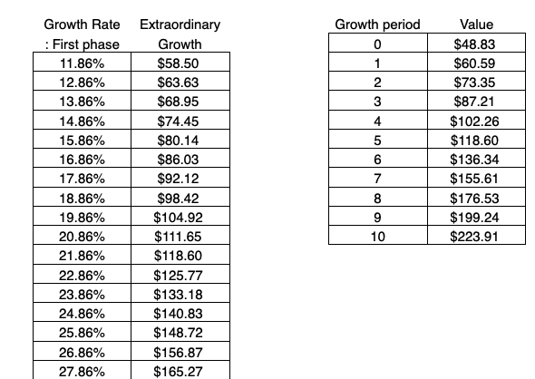 For instance, if your weighted average growth rate in the spreadsheet was 11.86%, you will be able to see the value of the high growth period at different percentages at 1% increments.
Conclusion
The dividend discount model is one of the most well-known valuation models and houses the basic mathematical framework for which discounted cash flows are traditionally constructed.
Although there are several inputs into the model, they can basically be boiled down to expected dividends and cost of equity. With that we can derive various output values that ultimately culminate in a projected stock price.
Like all models, the DDM has limitations in the degree to which it accurately reflects proper valuation estimates. Much of this lies in the Gordon Growth framework itself.
P = D / (r – g)
When the growth rate, g, increase toward the cost of equity, r, the price of the stock begins to increase exponentially. When the growth rate is very close to the cost of equity, the stock price approaches infinity.
If the growth rate exceeds the cost of equity, then the share price is negative.
Moreover, if a company does not pay dividends, the DDM projects its value as zero, since D (dividends value) is zero. Obviously, in these cases, the DDM is simply a bad fit.
However, the DDM can be especially useful for certain firms.
For firms that experience growth at approximately the same nominal rate as the economy, grow stably from year-to-year, and pay dividends up to their approximate capacity, the DDM will provide a reasonably robust estimation.
For firms that do not pay dividends up to their capacity, the DDM will underestimate the company’s share price.
The actual learning process starts by actually finding your way around these models on your own. The guides that are published are ideally reference material and background information.