Monte Carlo Simulations of Portfolio Growth (with Volatility & Leverage Variants)


Trading and investing isn’t about predicting or knowing the future. It’s about preparing for many possible ones.
Monte Carlo simulations let us stress-test portfolios by running thousands of “what if” scenarios with different volatility and leverage assumptions.
Instead of a single forecast, you see ranges of outcomes: steady growth paths, sudden collapses, and everything in between.
Most importantly, these simulations can also highlight the probability of “ruin” or simply unacceptable outcomes – the chance your capital falls below a critical threshold.
When we look at how leverage and market swings shape these odds, we can make smarter choices about risk, growth, and survival over the long run.
Key Takeaways – Monte Carlo Simulations of Portfolio Growth
- Monte Carlo simulations show ranges of outcomes, not single forecasts, making risk more visible.
- Diversified portfolios (with bonds) can handle modest leverage well, with very low ruin odds at 1.5x-2.0x.
- Bond-heavy allocations (like 60/40) stay resilient even with moderate leverage; only extreme leverage starts to hurt.
- Concentrated or highly correlated portfolios (e.g., heavy stocks + commodities, no bonds) collapse more quickly. Ruin risk spikes even at 2.0x.
- Leverage risk – as far as risk ruin – rises nonlinearly rather than gradually.
- Borrowing costs erode performance and can flip leveraged portfolios from winners to losers.
- Key findings: diversify broadly, use modest leverage only if you’re experienced/comfortable and following the idea of capital efficiency, and always manage for survival.
- This can fit both a trading and investing approach.
Setting Up the Simulations
Building the Portfolio
The starting point is a portfolio spread across five major asset classes/types: US stocks, international stocks, bonds, REITs, and commodities.
(Technically, REITs are also stocks and domestic/international stocks still heavily have the same type of environmental bias even if they’re split by geography.)
Each asset can be given its own expected return, volatility, and weight.
What we’ll do is look at how small changes in these assumptions or allocations reshape the overall portfolio profile.
Correlations between assets are also adjustable. This allows you to look at whether diversification holds up in different scenarios.
Adding Leverage and Costs
On top of the base portfolio, leverage levels can be dialed anywhere from half exposure to triple exposure.
Borrowing comes with a cost. Accordingly, the simulations include an annual cost of capital, so you can see the drag on performance when leverage is pushed too far. In this example, we use a 3% funding rate.
Time Horizon and Starting Capital
We sim out 50 years. Volatility, leverage, and time combine to shape very different paths.
Growth Paths Under Different Volatility Assumptions
Calm vs. Turbulent Markets
When volatility is low, the simulation will show portfolio paths clustering tightly around the median.
Growth is smoother, and ruin probabilities stay minimal.
In contrast, higher volatility spreads outcomes much wider. Some paths soar, but others go into loss territory.
We can quickly see how the same expected return can feel completely different depending on market stability.
Why Volatility Matters Beyond Returns
It isn’t just about how high the average return is. Volatility shapes the “journey” you go on along the way and creates more variance in the outcomes.
A portfolio with the same average return but double the volatility creates a much higher risk of hitting ruin early, even if the median outcome looks attractive.
What we see is that the left part of the distribution gets worse at higher percentiles the more leverage is applied.
For example, 20th-30th percentile outcomes may be worse at 3x leverage than 2x leverage.
The extent to which this occurs depends on the allocation.
This is where Monte Carlo shines: it makes risk visible, not just theoretical.
The Impact of Leverage
Amplified Gains and Losses
Leverage magnifies everything.
At modest levels and when used judiciously, it can make a portfolio grow faster, pushing median outcomes higher.
But as leverage increases, the spread between good and bad paths widens dramatically.
A lucky sequence of returns compounds wealth quickly, while a few early losses can wipe out years of progress.
The Trade-Off Readers Need to See
The simulations reveal that leverage isn’t a straight line between risk and reward.
Each extra turn of the dial brings disproportionately more downside risk.
At 1.5x leverage, ruin/unacceptable outcome odds may still feel manageable.
By 2x or 3x, the chance of catastrophic loss jumps, often overwhelming the benefit of higher potential returns.
There is a point where it’s just not worth it or you need to more conscientious of hedging against outcomes you can’t accept (which adds cost of its own).
Probability of Ruin
What “Ruin” Really Means
In the simulations, ruin is defined as your portfolio dropping below a set threshold – e.g., half of its starting value or another critical level where recovery becomes nearly impossible.
This isn’t bankruptcy in the legal sense, but it captures the point at which a long-term plan effectively fails.
How Volatility and Leverage Drive Ruin
As volatility increases, ruin probabilities rise, even without leverage.
Add leverage, and the jump is dramatic.
A portfolio that looks stable at 1x can see double-digit ruin odds at 2x-3x.
Sequence-of-Returns Risk
Timing matters. If losses strike in the first few years of a leveraged plan, the portfolio may never recover; even if average returns improve later.
The simulations make this danger tangible, showing how two investors with the same portfolio can end up in wildly different places depending on when good or bad years arrive.
What the Simulations Reveal
Median vs. Worst-Case Outcomes
The simulations highlight a key lesson: averages can mislead.
While the median path may look strong, the 10th percentile (or worse) often shows devastating losses.
Readers see that focusing only on the “typical” outcome hides the true range of risks.
The Nonlinear Nature of Risk
Risk doesn’t rise in a straight line.
Doubling leverage doesn’t just double the danger; it can significantly increase the probability of ruin.
This nonlinear effect is one of the most eye-opening insights from running thousands of scenarios.
Borrowing Costs Can Flip the Equation
Even if returns are decent, borrowing costs quietly erode performance.
At higher leverage, the drag becomes powerful enough to turn an attractive growth story into one where risk overwhelms reward. This hidden cost shows why leverage must be treated with caution.
Practical Takeaways
Setting a Personal Comfort Zone
The simulations make it clear that every investor has a tipping point.
One way to manage this is to decide on an acceptable probability of ruin (for example, less than 1% over 50 years) and adjust leverage so results stay within that boundary.
If you do choose to go beyond that, then it may require hedging, which involves its own cost.
Rethinking Diversification
Correlations often rise during crises – in the tails of distributions – reducing the safety net of diversification.
If possible, diversify with assets that behave differently in stress, not just during relatively calm markets.
Building Guardrails
Finally, the best defense is preparation.
Regular rebalancing, close monitoring of drawdowns, and preplanned steps to cut exposure when losses deepen all help keep a portfolio intact.
Results
Okay… with that said, let’s get into it.
Here are our assumptions/portfolio decisions.
US Stocks
- Expected Return: 7%
- Volatility: 16%
International Stocks
- Expected Return: 8%
- Volatility: 18%
Bonds
- Expected Return: 5%
- Volatility: 8%
REITs
- Expected Return: 8%
- Volatility: 20%
Commodities
- Expected Return: 4%
- Volatility: 22%
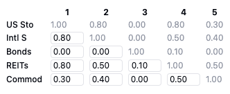
Correlation Matrix
Here are the correlations we set:
Base Portfolio Stats at 1x Leverage
Each simulation starts with $10,000 and runs for 50 years.
- Initial Capital: $10,000
- Expected Return: 6.3%
- Volatility: 10.8%
- Sharpe Ratio: 0.58
- Simulation Period: 50 years
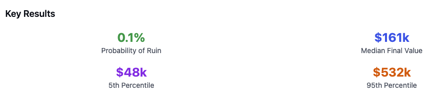
Allocation #1
- US Stocks – 25%
- International Stocks – 25%
- Bonds – 30%
- REITs – 5%
- Commodities – 15%
Leverage = 1.0x
This portfolio is diversified to the point where the probability of ruin – which we define as falling below $5,000 (we start with $10,000) – at any point is close to nil.
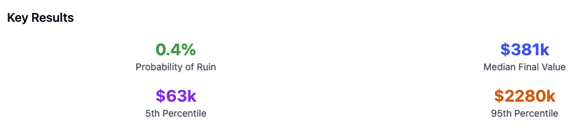
Leverage = 1.5x
Adding 1.5x leverage boosts the odds to 0.4%.
We do see improved results, especially at the median and upper percentile readings.
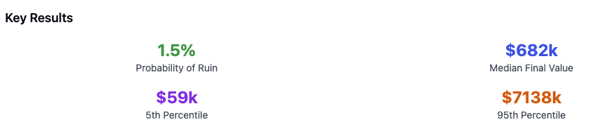
Leverage = 2.0x
This once again show the value of modest leverage.
5th percentile results are nonetheless lower than the 1.5x level.
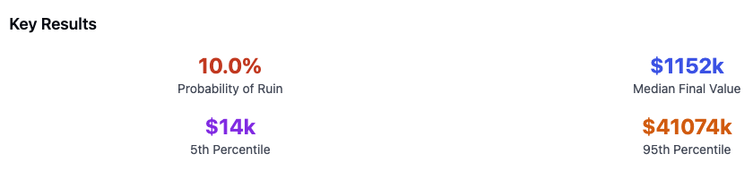
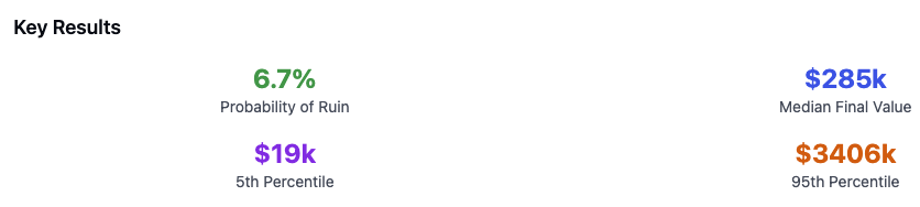
Leverage = 3.0x
3x leverage helps to boost median and 95th percentile outcomes (the latter in a nonlinear way).
The probability of bad outcomes is a bit high for conservative investors.
Allocation #2
- US Stocks – 25%
- International Stocks – 25%
- Bonds – 45%
- REITs – 5%
- Commodities – 0%
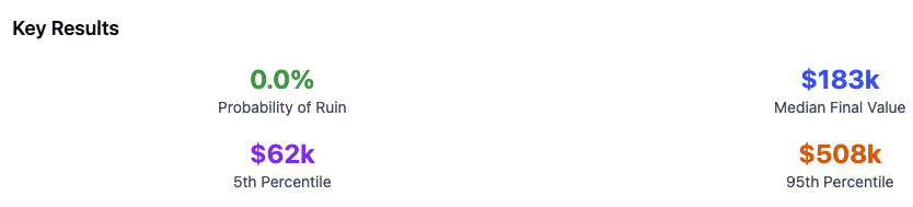
Leverage = 1.0x
This is a pretty standard portfolio – essentially 55% stocks and 45% bonds.
Unlevered, this portfolio is safe.
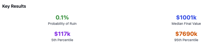
Leverage = 1.5x
Even at very modest leverage, this portfolio has very good results.

Leverage = 2.0x
Same…
Leverage = 3.0x
Here, we finally start seeing a little bit of pain in the lower percentiles.
The mid- and higher percentiles benefit.

Allocation #3
- US Stocks – 35%
- International Stocks – 35%
- Bonds – 0%
- REITs – 5%
- Commodities – 25%
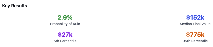
Leverage = 1.0x
Without the stability of bonds (and commodities and stocks go through periods of relatively high correlation), the probability of left-tail events is somewhat high with what’s essentially a 75% stocks and 25% commodities portfolio.
Leverage = 1.5x
With leverage, we see the left part of the distribution continue to suffer.
Leverage = 2.0x
Here we see a relatively high chance of wiping out at just 2x leverage.

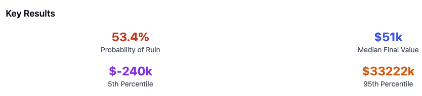
Leverage = 3.0x
At 3x leverage, the odds of wiping out are over 50%.
Even the median suffers significantly more than at 2x leverage.
This example shows the danger of leverage in concentrated – or highly correlated – portfolios.
Summary
Across the three allocations, the simulations show how diversification and leverage interact to shape both growth potential and risk of ruin.
Allocation #1 balances stocks, bonds, REITs, and commodities, resulting in a broadly diversified profile.
At 1.0x leverage, ruin risk is virtually zero.
Moderate leverage at 1.5x or 2.0x improves median and high-end outcomes with very limited additional risk, though by 3.0x the downside grows too large for conservative investors.
Allocation #2 is a classic 60/40-style mix tilted slightly more to bonds.
It’s very safe at 1.0x and performs strongly even at 1.5x and 2.0x leverage.
Only at 3.0x do the lower percentiles show real stress, though the upper percentiles benefit.
This highlights how bond-heavy allocations can safely absorb modest leverage.
Allocation #3 is concentrated in equities and commodities, with no stabilizing bond allocation.
Even unlevered, it carries higher left-tail risk due to correlations in downturns.
With leverage, losses accelerate quickly. 2.0x already shows significant wipeout risk, and 3.0x pushes the probability of ruin above 50%. Median outcomes also collapse.
The key lesson is clear: leverage can enhance returns when paired with diversification, but concentrated or correlated portfolios can implode under even moderate leverage.
Conclusion
Monte Carlo simulations don’t forecast or predict the market. They stress-test your decisions.
Running thousands of scenarios, you see how portfolios can thrive, stumble, or collapse under different conditions.
Portfolios behave with wide variance to them, leverage adds both speed and danger, and it’s important to frame choices in probabilities.
Most of all, it’s important to balance growth ambitions against the real risk of ruin, and protecting capital is the foundation for compounding over the long run.