Liquidity Models

Liquidity models are used in trading by assessing the ease with which assets can be bought or sold in the market without affecting their price.

These are several key concepts and liquidity model types that are important for traders, investors, and policymakers to understand – especially for traders who may impact markets with the sizes of their trades.

Notably, liquidity, market impact, transaction costs, and order execution are often ignored in many academic models despite their very important real-world effects.

Key Takeaways – Liquidity Models

• Market Depth and Impact
  • Liquidity models assess market depth and the potential price impact of trades.
  • Enables traders to predict and minimize slippage costs by adjusting order sizes and execution strategies in various market conditions.
• Adaptive Algorithms
  • These models use real-time data to adapt trading strategies.
  • Optimizes execution by dynamically adjusting to liquidity levels and market volatility.
  • Ensures more efficient trade execution.
• Cost-Benefit Analysis
  • Liquidity models provide a framework for a cost-benefit analysis of trading strategies.
  • Weighs the trade-off between execution speed and the cost of market impact.
  • Guides traders to make informed decisions on the timing and size of their trades.
• Liquidity Models & Optimal AUM Analysis
  • Liquidity models help in strategic decision-making regarding fund size, trading/investment strategies, and risk management.
    • Allows hedge funds and other institutional traders to optimize their returns while controlling for market impact and liquidity risk.
  • Transaction costs tend to rise in a non-linear way due to the diminishing availability of market liquidity for large orders, which causes disproportionate market impact and higher costs per additional unit of trade.
• Liquidity Model Coding Example
  • We simulate an order book to demonstrate a basic liquidity model with a visualization.

Here’s an overview of the key concepts and types of liquidity models:

Key Concepts

Market Liquidity

Refers to the ability to quickly buy or sell assets in the market at a price close to the market rate.

High liquidity is characterized by a high volume of trading and tight bid-ask spreads.

Funding Liquidity

The ease with which borrowers can obtain external financing.

It’s important during periods of financial stress when access to funding can become constrained.

Liquidity Risk

The risk that an entity will not be able to meet its financial obligations as and when they fall due because of an inability to liquidate assets or obtain funding.

Bid-Ask Spread

A measure of market liquidity.

The bid-ask spread is the difference between the highest price a buyer is willing to pay (bid) and the lowest price a seller is willing to accept (ask).

Narrower spreads generally indicate higher liquidity and lower transaction costs.

Depth

Indicates the volume of orders at different price levels in the market.

A market with depth can handle large orders without significant impact on the price.

Resiliency

The speed at which prices return to equilibrium after a large trade.

A resilient market quickly absorbs shocks and restores original price levels.

Types of Liquidity Models

Volume-Based Models

These models focus on the volume of trades and the available volume at different price levels to measure liquidity.

High trading volumes are generally associated with high liquidity.

Spread-Based Models

Assess liquidity by examining the bid-ask spread.

Narrow spreads are indicative of a more liquid market, as the cost to execute trades is lower.

Price-Impact Models

Estimate liquidity by measuring how much the price of an asset changes as a result of a trade.

Lower price impact suggests higher liquidity.

Part of LTCM’s failing was oversight of its price impact effects on markets.

Order Book Models

Analyze the depth and breadth of the market by studying the order book, which lists buy and sell orders at different price levels.

These models provide insights into market depth, tightness, and resiliency.

Time-Based Models

Consider the time it takes for a market to absorb a trade without affecting the asset’s price significantly.

Faster absorption rates indicate higher liquidity.

Composite Models

Combine multiple indicators of liquidity, such as volume, spread, and price impact, to provide a more comprehensive assessment of market liquidity.

Basic Math in Liquidity Models

Liquidity models in finance aim to quantify and analyze market liquidity using mathematical and statistical techniques.

Here are some of the key mathematical concepts involved:

Bid-ask spread

A narrower bid-ask spread indicates higher liquidity.

The relative bid-ask spread is calculated as:

Spread % = (Ask Price – Bid Price) / Mid Price

Trading volume

Higher trading volumes generally suggest greater liquidity.

The typical metric is daily or monthly trading volume.

Price impact

This measures how much prices move in response to trades.

Lower price impacts indicate higher liquidity/lower transaction costs.

It’s calculated as:

Price Impact = (P1 – P0) / P0

Where P1 is the price after a trade and P0 is the initial price.

Depth

Depth refers to the market’s ability to sustain large orders without substantial price changes.

It’s measured by the volume available at different bid and ask prices.

Resiliency

This refers to how quickly prices revert to previous levels after a large trade.

Faster reversion suggests higher liquidity.

Composite metrics

Models like the Amihud Illiquidity ratio combine multiple liquidity measures like spread, volume, and return to create an overall illiquidity score.

Illiquidity = |Return| / (Daily Volume x Mid Price)

Summary

The key mathematical techniques involve statistical metrics of volume, spreads, price changes, and order book depth and resiliency to quantify market liquidity.

These measures allow traders and regulators to better understand transaction costs and risks.

Coding Example – Liquidity Model in Trading

In this Python example, we’ve simulated an order book to demonstrate a basic liquidity model.

import numpy as np
import pandas as pd
import matplotlib.pyplot as plt

# Generate a simulated order book
np.random.seed(29)
order_prices = np.concatenate([np.random.normal(100, 0.5, 500), np.random.normal(100.5, 0.5, 500)])
order_sizes = np.random.randint(1, 10, 1000)
order_types = np.array(["Bid"]*500 + ["Ask"]*500)
order_book = pd.DataFrame({"Price": order_prices, "Size": order_sizes, "Type": order_types})

# Function to calculate liquidity measures
def calculate_liquidity_measures(order_book):
    bid_ask_spread = order_book[order_book['Type'] == 'Ask']['Price'].min() - order_book[order_book['Type'] == 'Bid']['Price'].max()
    depth = order_book.groupby('Type')['Size'].sum()
    return bid_ask_spread, depth

# Function to simulate a trade and its impact on liquidity
def simulate_trade(order_book, trade_size, trade_type):
    if trade_type == "Buy":
        available_liquidity = order_book[order_book['Type'] == 'Ask'].sort_values(by='Price')
    else: # Sell trade
        available_liquidity = order_book[order_book['Type'] == 'Bid'].sort_values(by='Price', ascending=False)

    cumulative_liquidity = available_liquidity['Size'].cumsum()
    price_impact_point = available_liquidity[cumulative_liquidity >= trade_size].iloc[0]
    price_impact = price_impact_point['Price'] - (order_book[order_book['Type'] == 'Bid']['Price'].max() if trade_type == "Buy" else order_book[order_book['Type'] == 'Ask']['Price'].min())

    return price_impact

# Calculate initial liquidity measures
initial_bid_ask_spread, initial_depth = calculate_liquidity_measures(order_book)
print(f"Initial Bid-Ask Spread: {initial_bid_ask_spread}")
print(f"Initial Market Depth: {initial_depth.to_dict()}")

# Simulate a buy trade
buy_trade_size = 50
buy_price_impact = simulate_trade(order_book, buy_trade_size, "Buy")
print(f"Price Impact of a {buy_trade_size} Size Buy Trade: {buy_price_impact}")

# Simulate a sell trade
sell_trade_size = 50
sell_price_impact = simulate_trade(order_book, sell_trade_size, "Sell")
print(f"Price Impact of a {sell_trade_size} Size Sell Trade: {sell_price_impact}")

# Visualize the order book
plt.figure(figsize=(10, 6))
plt.hist(order_book[order_book['Type'] == 'Bid']['Price'], bins=30, alpha=0.5, label='Bids')
plt.hist(order_book[order_book['Type'] == 'Ask']['Price'], bins=30, alpha=0.5, label='Asks')
plt.legend()
plt.title('Simulated Order Book')
plt.xlabel('Price')
plt.ylabel('Number of Orders')
plt.show()

Results

Here’s a summary of the results and visualization:

• The initial bid-ask spread was calculated as approximately -2.77.
  • Indicates the difference between the minimum asking price and the maximum bidding price in our simulated order book.
• The market depth, showing the total size of bids and asks, was 2482 for bids and 2532 for asks.
  • Highlights the volume available at different price levels.
• Simulating a buy trade of 50 units resulted in a price impact of approximately -2.45.
  • Shows how much the price would potentially move against the buyer.
• Similarly, simulating a sell trade of 50 units had a price impact of approximately 1.92.
  • Reflects the potential price movement against the seller.

Statistics for bid-ask, market depth, price impact

• The histogram visualizes the distribution of bid and ask orders to show the simulated market depth and the bid-ask spread.

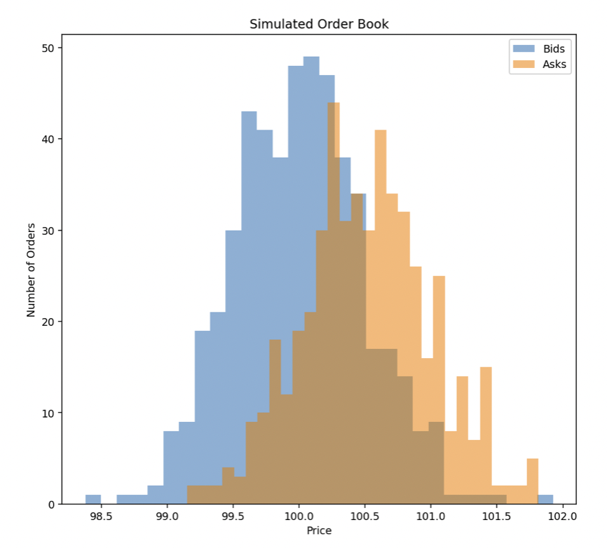
This simple model showcases how traders can use liquidity measures to assess the impact of their trades and make informed decisions based on market depth and price movements.

Liquidity Models & Market Microstructure

Liquidity models and market microstructure provide insights into how securities are traded and prices are formed in financial markets.

These models dissect the impact of:

• order flow
• bid-ask spreads
• trading volume, and
• market participants’ behavior on liquidity…

…studying the mechanisms behind price discovery and execution efficiency.

They explore the dynamics between market makers, high-frequency traders, and institutional traders/investors, revealing how each contributes to or detracts from market liquidity.

By understanding the microstructural elements, such as the role of electronic trading platforms, the regulatory environment, and the introduction of new financial instruments, liquidity models can predict how changes in market structure affect liquidity.

This knowledge enables traders and policymakers to make better decisions, whether it’s executing large orders without causing significant price impact or shaping regulations to enhance market stability and efficiency.

Related: Market Microstructure & Algorithmic Trading

Liquidity Models for Market Makers

Market makers use liquidity models to determine the optimal width of bid-ask spreads and the depth of orders they should provide on both sides of the market.

These models help them manage inventory risk by predicting short-term price movements and volume flows.

This enables them to adjust their positions to maintain profitability while providing liquidity.

The models factor in the cost of carrying inventory and the potential adverse selection risk, guiding market makers on when to adjust their quotes to minimize losses and maximize the spread benefits.

Market makers make money by buying securities at a lower price (the bid) and selling them at a higher price (the ask), profiting from the spread between these two prices while providing liquidity to the market by being ready to buy or sell at any time.

Liquidity Models for High-Frequency Traders (HFTs)

High-frequency traders utilize liquidity models to identify fleeting opportunities in order execution imbalances and price discrepancies across markets or instruments.

These models help HFTs to execute large volumes of trades at high speeds, capitalizing on small price movements with minimal impact costs.

They analyze historical and real-time data to predict liquidity patterns, allowing HFTs to strategically place orders that are likely to be filled quickly at favorable prices.

The emphasis is on speed and the ability to anticipate short-term liquidity fluctuations, leveraging technology to automate and optimize trading strategies for thin margins at a high volume.

Related: HFT Strategies

Liquidity Models & AUM Determination for Institutional Traders and Investors

Liquidity models are used by hedge funds in determining their optimal asset under management (AUM) size, as these models assess the market’s ability to absorb trade volumes without significant price impact.

By analyzing market depth, bid-ask spreads, and the price impact of trades, liquidity models enable hedge funds to estimate the maximum trade size that can be executed while minimizing slippage costs.

This analysis helps hedge funds to gauge the scale of trades, positions, and investments they can manage effectively before their trades begin to adversely affect market prices (to ensure that they can enter and exit positions efficiently).

Transaction costs tend to increase in a non-linear way because larger trade sizes not only affect the bid-ask spread but also require deeper market liquidity, which can significantly impact the price and lead to higher costs per unit traded as order size increases.

Conclusion

Understanding these concepts and models is important for financial market participants, as liquidity affects trading strategies, asset valuation, and risk management practices.

It also has implications for financial stability and regulatory policies, especially during periods of market stress when liquidity can evaporate, which can lead to broader systemic risks.