Time Series Forecasting Models in Trading


Time series forecasting models in trading are statistical techniques used to predict future values of financial assets based on historical data.
These models try to identify patterns and trends in time series data to help traders to make informed decisions about entry and exit points, as well as risk management strategies.
Accurate forecasting can provide a competitive edge in the markets, but it’s important to continuously validate and refine these models and combine them with other forms of analysis.
Key Takeaways – Time Series Forecasting Models
- Moving Averages (MA)
- Simple Moving Averages (SMA)
- Exponential Moving Averages (EMA)
- Autoregressive Integrated Moving Average (ARIMA)
- Exponential Smoothing
- Simple Exponential Smoothing (SES)
- Holt-Winters Exponential Smoothing
- Holt’s Trend Method
- Generalized Autoregressive Conditional Heteroskedasticity (GARCH)
- Recurrent Neural Networks (RNNs) and Long Short-Term Memory (LSTM)
- Vector Autoregression (VAR) and Vector Error Correction Model (VECM)
- VAR
- VECM
- Markov Switching Models
- Wavelet Analysis
- Seasonal Decomposition of Time Series (STL)
- Prophet
- Neural Networks and Machine Learning
- Recurrent Neural Networks (RNNs)
- Long Short-Term Memory Networks (LSTMs)
- Other models
- Applications in Trading
- Price Prediction
- Trend Analysis
- Volatility Forecasting
- Algorithmic Trading
- Coding examples below
Moving Averages (MA)
Moving averages are well-known and represent simple time series.
Simple Moving Averages (SMA)
Calculates the average price over a specified period to identify trends and potential support/resistance levels.
Exponential Moving Averages (EMA)
Similar to SMA but gives more weight to recent prices, making it more responsive to new information.
Autoregressive Integrated Moving Average (ARIMA)
Combines autoregressive and moving average components to model time series data, particularly effective for non-stationary data after differencing.
Exponential Smoothing
Simple Exponential Smoothing (SES)
Focuses on the most recent data points to make forecasts, suitable for data with no clear trend or seasonal pattern.
Holt-Winters Exponential Smoothing
Extends SES to handle data with trends and seasonality.
Holt’s Trend Method
Captures trends within the data.
Generalized Autoregressive Conditional Heteroskedasticity (GARCH)
Models volatility in financial time series, capturing the time-varying nature of volatility for options pricing and risk management.
Recurrent Neural Networks (RNNs) and Long Short-Term Memory (LSTM)
Deep learning models that are effective for forecasting complex and non-linear time series data, capturing long-term dependencies.
Vector Autoregression (VAR) and Vector Error Correction Model (VECM)
VAR
Captures interdependencies between multiple time series variables.
VECM
Used when variables are cointegrated, indicating a long-term equilibrium relationship.
Markov Switching Models
Account for regime shifts or structural breaks in time series data, useful for capturing market cycles and trading regime changes.
Wavelet Analysis
Decomposes time series into various frequency components for analyzing and forecasting patterns at different time scales.
Seasonal Decomposition of Time Series (STL)
Decomposes a time series into seasonal, trend, and residual components, useful for time series with strong seasonal patterns.
Prophet
Developed by Facebook for forecasting with daily observations that display patterns on different time scales, robust to missing data and trend shifts.
Neural Networks and Machine Learning
Recurrent Neural Networks (RNNs)
Designed for time series data, retaining information from previous time steps.
Long Short-Term Memory Networks (LSTMs)
A type of RNN capable of handling long-term dependencies.
Other models
Include XGBoost and Random Forests for time series forecasting.
Applications in Trading
Price Prediction
Traders often try to forecast future asset prices to make informed buy/sell decisions.
Trend Analysis
Identifying underlying trends (upward, downward, sideways) to develop trading strategies.
Volatility Forecasting
Assessing future asset price volatility to manage risk and optimize trading positions.
Algorithmic Trading
Time series models are core components of automated trading systems that make trades based on data analysis.
Considerations
Stationarity
Many traditional time series models assume the data is stationary. Traders often transform non-stationary data before applying these models.
Complexity
Neural networks and machine-learning models offer greater flexibility but can be more challenging to interpret.
Fundamental Analysis
It’s essential to remember that time series models solely rely on historical price data. It’s best to combine their insights with fundamental analysis, which examines a company’s financial health, industry, and broader economic factors.
Improving Time Series Models
These models, which include ARIMA, GARCH, and others, traditionally rely on statistical and mathematical theories to forecast future values based on past observations.
Despite their widespread use, time series models in finance exhibit several limitations:
Linear Assumptions
Many time series models assume a linear relationship between past and future values, often overlooking the complex, non-linear dynamics in financial markets.
Stationarity Requirement
These models generally require the data to be stationary, meaning its statistical properties do not change over time.
However, financial data often exhibit trends, volatility clustering, and structural breaks, challenging this assumption.
Historical Data Dependence
Time series analysis heavily relies on historical data.
In rapidly changing environments, like financial markets, past patterns may not reliably predict future movements, especially in the face of unprecedented events or shifts in market dynamics.
Limited External Factor Integration
Traditional models may not adequately incorporate external factors or qualitative information, such as changes in regulations, market sentiment, or geopolitical events, which can significantly impact financial outcomes.
Time Series Enhancement
Times series are based on only historical data, and predicting the future based on historical data is generally not robust enough on its own.
You’ll generally need to provide other forms of analysis.
Let’s take large language models as an example.
LLMs offer a new way for addressing the inherent limitations of traditional time series models in finance by leveraging their ability to have read virtually everything that’s been written and writing/theorizing about the data it’s been fed.
Here’s how LLMs can complement and enhance time series analysis:
Incorporating Qualitative Data
LLMs can analyze vast amounts of qualitative data, such as news articles, financial reports, and social media sentiment, integrating external factors that significantly influence financial markets.
Complex Pattern Recognition
Through deep learning, LLMs can identify complex, non-linear patterns within large datasets, capturing relationships that traditional time series models may miss.
Dynamic Model Adaptation
LLMs can continuously learn from new data, allowing models to adapt to changing market conditions more dynamically than static, historically dependent models.
Scenario Analysis and Simulation
By generating text-based scenarios, LLMs can simulate various future states of the world, offering a richer set of possibilities for stress testing and scenario analysis beyond the constraints of historical data.
Coding Example #1 – LSTM Time Series on Cyclical Data
Designing a Long Short-Term Memory (LSTM) model for time series analysis involves data preprocessing, model construction, and training.
Here’s a high-level outline of how you could design an LSTM model for time series forecasting:
1. Data Preprocessing
- Collect Data – Time series dataset with consistent time intervals (e.g., daily, monthly).
- Clean Data – Handle missing values, remove outliers, and ensure the data quality is good for model training.
- Normalize Data – Scale the data to a specific range (often 0 to 1) to improve the LSTM model’s convergence speed and stability.
- Sequence Creation – Convert the time series into a supervised learning problem. For example, use previous time steps as input variables to predict the next time step(s).
2. Model Construction
Define Model Architecture:
- Input Layer – Define the shape (number of time steps and features per step).
- LSTM Layer(s) – Choose the number of LSTM units (neurons). Multiple layers can increase the model’s ability to capture complex patterns.
- Dropout Layer(s) – Optional, to prevent overfitting by randomly dropping units from the neural network during training.
- Output Layer – Typically one neuron for univariate forecasting or more for multivariate forecasting.
Compile Model:
- Loss Function – Mean Squared Error (MSE) or Mean Absolute Error (MAE) are common for regression problems.
- Optimizer – Adam, SGD, or others to minimize the loss function.
3. Model Training
- Train-Test Split – Divide the data into training and testing sets to evaluate the model’s performance.
- Fit Model – Train the model using the training data, specifying the number of epochs (iterations) and batch size.
- Validation – Use a portion of the training data or separate validation data to tune hyperparameters and prevent overfitting.
4. Model Evaluation and Testing
- Evaluate Performance – Use the test data to evaluate the model’s performance, typically using metrics like RMSE (Root Mean Squared Error), MAE, etc.
- Parameter Tuning – Adjust model parameters based on performance metrics to improve accuracy and reduce overfitting.
5. Prediction and Deployment
- Forecasting – Use the model to make predictions on new data.
- Deployment – Integrate the model into a production environment for real-time or batch forecasting.
Here’s some example code of how LTSM can be good for cyclical patterns (be sure to have the relevant libraries installed):
import numpy as np
import matplotlib.pyplot as plt
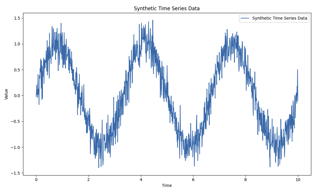
# Generate synthetic time series data (sinusoidal/cyclical pattern)
t = np.linspace(0, 10, 1000) # Time variable
data = np.sin(2 * np.pi * 0.3 * t) + np.random.normal(scale=0.2, size=t.shape) # Sinusoidal data with noise
# Plot the synthetic time series data
plt.figure(figsize=(10, 6))
plt.plot(t, data, label='Synthetic Time Series Data')
plt.title('Synthetic Time Series Data')
plt.xlabel('Time')
plt.ylabel('Value')
plt.legend()
plt.show()
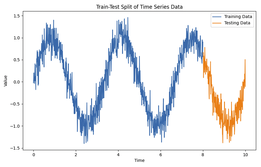
# Train-test split
train_size = int(len(data) * 0.8)
test_size = len(data) - train_size
train_data, test_data = data[0:train_size], data[train_size:len(data)]
# Time split for plotting
train_time, test_time = t[0:train_size], t[train_size:len(t)]
# Plot training and testing data
plt.figure(figsize=(10, 6))
plt.plot(train_time, train_data, label='Training Data')
plt.plot(test_time, test_data, label='Testing Data')
plt.title('Train-Test Split of Time Series Data')
plt.xlabel('Time')
plt.ylabel('Value')
plt.legend()
plt.show()
from tensorflow.keras.models import Sequential
from tensorflow.keras.layers import LSTM, Dense
# Assuming data is prepared appropriately for LSTM (scaled, sequenced, etc.)
# Here we use the data directly for simplicity; in practice, you should preprocess it
# Model definition
model = Sequential()
model.add(LSTM(units=50, return_sequences=False, input_shape=(1, 1)))
model.add(Dense(1))
model.compile(optimizer='adam', loss='mean_squared_error')
# Assuming X_train and y_train are created from the train_data
model.fit(X_train, y_train, epochs=10, batch_size=1)
# Hypothetical predictions from the model
predictions = model.predict(X_test)
# Plot results
plt.figure(figsize=(10, 6))
plt.plot(test_time, test_data, label='True Test Data')
plt.plot(test_time, predictions, label='Predicted Data')
plt.title('LSTM Model Predictions vs True Data')
plt.xlabel('Time')
plt.ylabel('Value')
plt.legend()
plt.show()
The greater the number of epochs* the slower the code will be. We did just 10 to speed it up at the trade-off of less accuracy.
*An epoch in LSTM training is one complete pass through the entire training dataset during which the model’s weights are updated.
Results
Here’s our synthetic time series data:
And here’s how the training data fits the testing data (i.e., picks up what the data is all about and predicts it well):
Coding Example #2 – LTSM for Stock Price Predictions
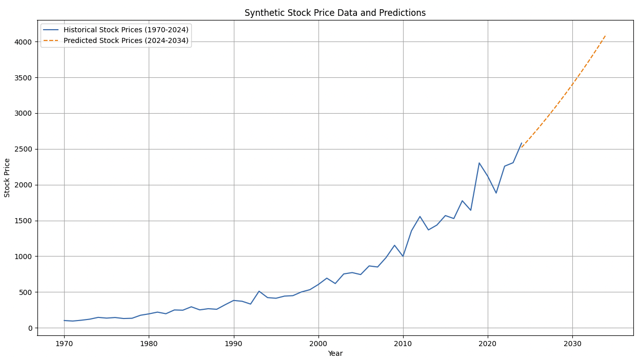
Let’s say we wanted to study a stock that has data from 1970 to the beginning of 2024 and we want to use that data to predict performance for the stock from 2024-2034.
We’re going to use synthetic data and make sure it represents a stock accurately by having a drift factor + a volatility component. (Related: Stochastic Differential Equations in Trading)
To create and train an LSTM model for predicting stock prices in this way, we would typically follow these steps:
- Generate synthetic stock data. Use real data for real-world cases.
- Preprocess the data for the LSTM model.
- Define the LSTM model architecture.
- Compile and train the model.
- Compile the model using a loss function (e.g., mean squared error) and an optimizer (e.g., Adam).
- Train the model using the training data.
- Evaluate the model’s performance on the testing data.
- Predict what you want to predict.
- Evaluate the model’s performance.
Here’s how the code might look:
import numpy as np
import pandas as pd
import matplotlib.pyplot as plt
from sklearn.linear_model import LinearRegression
from sklearn.preprocessing import PolynomialFeatures

# Generate synthetic stock price data from 1970-2024
np.random.seed(153)
years = np.arange(1970, 2025)
trend = 100 * (np.exp(0.06 * (years - 1970))) # Exponential growth to simulate stock price increase
volatility = np.random.normal(0, 0.1, len(years)) * trend # Volatility as a percentage of the trend
stock_prices = trend + volatility

# Fit a polynomial regression model
X = years.reshape(-1, 1)
y = stock_prices
poly = PolynomialFeatures(degree=4)
X_poly = poly.fit_transform(X)
model = LinearRegression()
model.fit(X_poly, y)

# Predict stock prices from 2024-2034
future_years = np.arange(2024, 2035)
future_X = future_years.reshape(-1, 1)
future_X_poly = poly.transform(future_X)
predicted_prices = model.predict(future_X_poly)

# Combine historical & predicted data for plotting
all_years = np.concatenate((years, future_years))
all_prices = np.concatenate((stock_prices, predicted_prices))

# Plot stock price data and the predictions
plt.figure(figsize=(15, 8))
plt.plot(years, stock_prices, label='Historical Stock Prices (1970-2024)')
plt.plot(future_years, predicted_prices, label='Predicted Stock Prices (2024-2034)', linestyle='--')
plt.title('Synthetic Stock Price Data and Predictions')
plt.xlabel('Year')
plt.ylabel('Stock Price')
plt.legend()
plt.grid(True)
plt.show()
Results
Important Points
- Time series forecasting models are just one analysis method. They give you probabilities, not outright guarantees.
- Backtesting on historical data is important before using any model in real-world trading.
- It doesn’t necessarily show future performance, but always know something’s track record.
- Markets are influenced by many factors, some hard to quantify – time series analysis is just one form of analysis.