An Overview of the Leveraged Buyout (LBO) Financial Model

A leveraged buyout (LBO) is a transaction where a financial sponsor purchases a company or specific asset with equity and substantial amounts of borrowed capital.

The target company being acquired has its assets and cash flows used as leverage in the buyout to obtain and finance the deal.

The LBO is a common transaction form for private equity firms, where high levels of debt are used to leverage transactions.

Nonetheless, there is always an element of risk inherent in each transaction. If a transaction is over-leveraged, and assets and cash flows are not sufficient to service the debt, insolvency of the business can ensue.

Private equity firms and banks form a mutually beneficial relationship in LBO deals.

The private equity firm can generate a substantial return on equity by leveraging high levels of debt while the bank can improve its profit margins by providing the funding debt for the LBO given the profits from net interest income (NII) over standard corporate lending.

Yet the bank on the same token has to manage its risk in accordance to:

• the value of the company or asset being purchased
• the financial profile of the private equity firm
• the equity the firm can provide, and
• the pre-existing quality of the current economic environment

Large firms inherently have a greater advantage over middle market and smaller private equity firms in securing the best rates and establishing the strongest relationships with banks.

For targeted companies with strong, relatively non-volatile cash flow, up to 100 percent of the purchase price can be provided via debt volume. More typical ratios are 50 percent of the purchase price.

Characteristics of good leveraged buyout (LBO) targets

Private equity firms look for a few distinct characteristics when considering what companies would become quality targeted buyout candidates.

Prospective deals may be looked into when private equity research points to the following traits:

• Strong, stable cash flows (as mentioned)
• Companies that are undervalued, or at least appropriately valued
• Low fixed costs
• Low debt balance
• Strong management/decision-making team

Basic LBO Model

With the basic idea behind leveraged buyouts in mind, let’s delve into a basic LBO model. The model I will be using is adapted from Wall Street Prep and is very basic (it can be found here).

Most of it is the same free model that they provide, but with certain modifications made such that it flows a bit more logically. It is by no means a comprehensive model, but is rather used for education purposes only.

The idea is to first understand how the basic structure of an LBO model works, and how manipulating the basic inputs influences key outputs, such as:

• The EV/EVITDA multiple (technically an input, but determined from more basic inputs)
• Enterprise value in the exit year
• Equity values in the exit year
• Maximum amount that can be financially invested into the bought out firm
• Funds available to acquire firm and pay off its debt
• Highest purchase price sponsor would be willing to pay for the target company’s shares

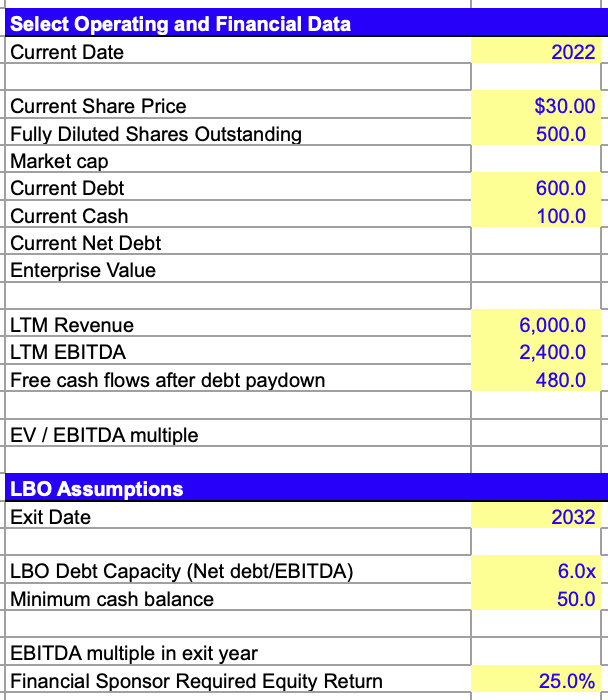
The LBO Model: Inputs

An LBO model is specified by a date. Both the date when the transaction will be completed followed by an exit date where all debt will be paid down on the transaction.

Next, we look at the share price of the company prospectively being purchased.

Then the number of fully diluted shares outstanding. Diluted shares refer to all forms of stock that can be transformed from other convertible forms of stock, including warrants, stock options, and convertible bonds.

This helps to better assess financial performance over undiluted shares, which are merely stock in its common form.

From these inputs, we can determine market cap:

Market Cap = Current Share Price x Fully Diluted Shares Outstanding

From here, we input the current debt and cash values of the firm.

From this, we determine net debt, equal to:

Net Debt = Current Debt – Current Cash

And from the combination of the basic four outputs we’ve mentioned thus far, we can determine enterprise value.

Enterprise value (EV) is equal to the sum of the two second-order inputs we’ve derived from our initial four first-order inputs:

EV = Market Cap + Current Net Debt

This is an oversimplification of enterprise value. It’s more appropriately valued with several additional inputs that must go into “current net debt” but will suffice for this exercise.

Next, we look at the revenue from the last twelve months of the firm (LTM Revenue).

We also look at things like earnings before interest, taxes, depreciation, and amortization (EBITDA). This helps to compare companies by subtracting out various parameters to control for their effects.

Namely, when we take out the “ITDA” from EBITDA, we control for:

• forms of financing (interest payments)
• jurisdiction/tax bracket effects (taxes)
• asset collection (removes depreciation), and
• takeover history (by eliminating amortization from intangible assets like patents or brand name).

A negative EBITDA denotes issues with profitability and cash flow. EBITDA may denote profitability but does not imply positive cash flow as it inherently ignores changes in taxes, interest, working capital, and capital expenditures.

Next, we determine free cash flow.

Cash flow in itself refers to the process of cash in and out of a firm through its operations.

Free cash flow is the cash flow available to be distributed to its securities holders without negatively impacting operations.

Free cash flow can be determined a few different ways and necessitates access to the company’s income statement and balance sheet. One such method:

FCF = EBIT (1 – tax rate) – D&A – Working Capital – Capital Expenditures

Free cash flow cannot be calculated from the income statement alone given working capital is a necessity and must be obtained from the balance sheet.

Working capital entails two of the three main components of a balance sheet by subtracting liabilities from assets.

Alternative ways to calculate free cash flow with just working capital and income statement items include:

FCF = EBIT (1 – t) + D&A – ∆Working Capital – Investment in operating capital

FCF = Net income + Interest expense – Net capex – Net ∆Working Capital – Tax shield on interest expense

For simplicity purposes in our model, free cash flow is a basic input.

For our final input, we combine first-order inputs in EV and EBITDA to form a valuation multiple by dividing the two to form EV/EBITDA.

This determine enterprise value per every unit of earnings controlled for the aforementioned factors. EV/EBITDA helps to compare valuation across multiple companies with varying debt levels as it controls for capital structure.

(Capital structure refers to how a corporation finances its assets – equity, debt, or hybrid securities. From a theoretical point of view, the Miller-Modigliani theorem asserts that how a firm is financed has no relation to its value; however, the prices of different forms of financing matters.)

From EV/EBITDA we generate a valuation multiple.

Lower EV/EBITDA companies are considered better buys than higher EV/EBITDA companies.

For a lower EV/EBITDA company, it suggests that we will be paying less for our cash flow over a higher EV/EBITDA company.

If we have a relatively low numerator (EV) but a high denominator (EBITDA), the resultant valuation will be relatively high.

Consequently, this may suggest that we will be paying a relatively low amount for our cash flow for a company that has high potential growth.

Assumptions

Here we’ll include an exit date right off the bat. Usually, the difference between a start date and exit date of a leveraged buyout deal is 4-10 years, although it depends.

For simplicity, we’ll say current and exit dates are on December 31 of their respective years to keep it in terms of whole years and have our fiscal year dovetail with the start and end of the calendar year.

For our model, we must make certain assumptions:

• LBO Debt Capacity (Net debt / EBITDA)
• Minimum cash balance
• EBITDA multiple in exit year
• Sponsor’s required equity return

The debt capacity of the LBO is represented through the Net debt / EBITDA metric. This is essentially a measure of leverage.

It’s a measure of how the debt relates to the operational capacity of the firm via its earnings controlled for interest, taxes, depreciation, and amortization.

The leverage ratio becomes risky beyond a certain point.

In private equity, the net debt / EBITDA metric is normally kept below three although it largely depends.

The default that was programmed into this LBO template was six, which is much too high for most firms due to the unhealthy degree of risk involved.

If a firm is leveraged 6x, that means only a 10 percent adverse change in equity value would reduce its value by 60 percent. A drawdown of more than about 17 percent would produce a negative net worth.

Leverage is a double-edged sword. While it allows you to scale up profits quickly, it also does the exact same thing in reverse if the deal doesn’t work out entirely.

For a minimum cash balance, there needs to be some benchmark. You can place it at about one percent of revenue, or 2.5 percent of EBITDA.

It could also be set to zero for maximum flexibility for a firm, although it does not influence the deal’s likelihood of occurring.

Select Operating and Financial Data

Here we will track the following variables through calculations:

• Projected revenue
• Revenue growth
• EBITDA
• EBITDA margin
• FCF after required debt pay down
• FCF margin percentage

Revenue is placed in from our earlier input. The revenue growth rate (annual) is also input on our own.

It will assume a constant rate of growth during the course of the debt pay down (i.e., from when the deal was initiated to when the debt is paid off).

If we plug in 10 percent, for example, the firm will grow by 10 percent each year through the course of the debt servicing.

The nominal rate of growth for the US or any large fiscally stable country is normally 2 to 5 percent. Estimates for firms of private equity buyouts will generally be higher, given the idea is to get the company on the appropriate business track in the first place.

Consequently, the firm more growth more swiftly at first before maturing into a stable growth pattern.

EBITDA was input earlier (technically LTM EBITDA, given we are taking data from just the last twelve months).

EBITDA margin describes EBITDA as a percentage of its total revenue:

EBITDA Margin = EBITDA / Total Revenue

Given EBITDA is a proxy for cash flow, EBITDA margin denotes how much cash came in the form of total revenue. The higher, the better for evaluation purposes.

EBITDA Shortcomings

Note that while EBITDA is popular, it possesses its own shortcomings.

It’s largely unsuitable for firms with:

• low net income (because EBITDA will usually overstate its degree of profitability)
• high levels of debt, or
• those with high rates of depreciation (leading to a high rate in equipment turnover).

Also, EBITDA isn’t regulated by GAAP accounting regulations.

Hence, companies can use their own modifications and adjustments to manipulate the value.

Companies can also technically produce a high EBITDA for many years yet have capital expenditures exceeding cash flow, causing bankruptcy. (Capital expenditures aren’t included within the EBITDA calculation.)

Free Cash Flow (FCF)

Free cash flow is placed into this category directly from our earlier inputs.

Also, we include FCF margin, which is equal to:

FCF Margin = FCF / Total Revenue

Also, in this case, the higher free cash flow margin the better in terms of company financial health.

In sum, it determines how many cents out of every dollar ends up being distributed back to shareholders.

You can make an argument that FCF margin is the single most important financial metric during a recession. It will ultimately help measure how safe and sustainable a business is.

Debt Schedule

A debt schedule is part of an LBO model.

Below is a simplified representation, but it basically involves using the cash flow of the firm to pay down the debt that was used to help acquire the firm.

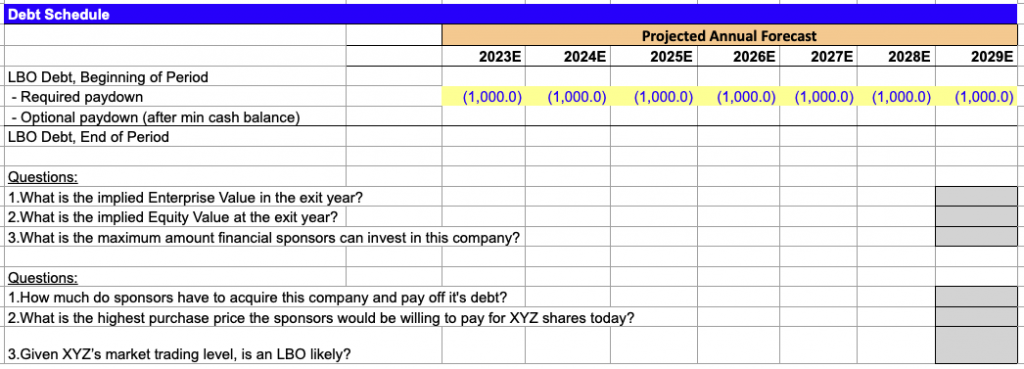
Our debt schedule gives us information on how much debt we start with at the start date, our required pay down each year (this is assumed) and our degree of optional debt servicing.

The amount of debt we can start with is a function of LTM EBITDA (EBITDA within the last twelve months) and our LBO debt capacity, dictated by the Net debt/EBITDA ratio.

For instance, if we start out with $25 million for our LTM EBITDA and have a net debt/EDITDA ratio of 4, then our LBO debt at the beginning of the period would be $100 million.

This $100 million would decrease according to the terms of the pay down agreement (i.e., pay off the debt in quantities of X amount per month or year).

We would also have optional pay down, which we calculate from our basic inputs:

Optional pay down = (Cash + Free cash flow after required pay down – Minimum cash balance)

LBO debt at the beginning of the period is equal to:

LBO debt, end of period = LBO debt, beginning – Required pay down – Optional pay down

Then we have the change in cash and debt over the time period, which in turn determines changes in net debt over the time period.

This is determined directly from the debt schedule. (Cash – Debt = Net Debt)

Deriving Outputs

In the output section of an LBO model, we will typically derive the following:

• Implied enterprise value in the exit year
• Implied equity value in the exit year
• Maximum amount financial sponsors (i.e., private equity firm) can invest in this company
• The amount available to acquire this company
• The highest purchase price the sponsors would be willing to pay for the target firm’s shares
• Likelihood of a leveraged buyout occurring, based on an index

The implied enterprise value in the exit year can be derived using the HLOOKUP function in excel.

This will allow us to derive the enterprise value of the firm based off the exit date specified in our “Assumptions” section.

HLOOKUP will derive the enterprise value by searching for the appropriate row where EBITDA is found and take the value in the cell matching up with the exit date specified.

If we have an exit date on the deal specified as the year 2032, then HLOOKUP will take the value of EBITDA in the year 2032 and then multiply by our EV/EBITDA multiple.

When EBITDA and EV/EBITDA are multiplied together, EBITDA cancels out and we are left with EV.

For implied equity value in the exit year, we also use HLOOKUP. Implied equity value is a function of net debt subtracted from enterprise value.

So we specify the row where net debt is, and HLOOKUP will find the value for the specific exit year. When this value of net debt is subtracted from EV, we derive our implied equity value in the exit year.

The maximum amount financial sponsors can invest in the company being potentially acquired relates to how much capital the private equity firm is willing to invest in the company.

This is a function of the implied equity value in the exit year, the equity return required by the financial sponsor, and the length of the LBO deal.

We calculate this accordingly:

Maximum invested in company = (Implied Equity Value in exit year) / (1 + Required Equity Return) ^ (Exit Year – Current Year)

The amount available to acquire the company and pay off its debt is equal to the previous value (maximum amount available to invest in company) added to the debt at the beginning of the period.

The highest purchase price the sponsors would be willing to pay for the company’s shares is equal to:

Highest Price for Company’s Shares = [(Amount available to acquire company and pay off its debts) – (Nebt Date, beginning)] / (Fully Diluted Shares Outstanding)

And finally, the likelihood of the LBO depends on whether the highest price the sponsors are willing to pay for the company’s share exceeds that of the company’s current share price.

How Inputs Affect Outputs

After placing in our inputs, the bulk of the actual learning portion can actually begin in the form of how manipulating our inputs affect our outputs.

This is where we can begin to understand how the actual math of an LBO model functions.

An increased market cap decreases the likelihood of an LBO deal from occurring because the company simply costs more to acquire.

A decreased market cap (share price multiplied by fully diluted shares outstanding) proportionally increases the ratio between the highest purchase price sponsors would be willing to pay for the shares versus the current share price.

The more debt the firm has, the lower the likelihood of an LBO (greater debt denotes a lesser degree of financial health).

On the flip side the more cash a firm has on hand, the greater the possibility of a deal (better financial health).

In sum, the less net debt the company has through a combination of less debt and/or more cash, the more feasible an LBO deal is.

A higher free cash flow after debt pay down has a positive effect on likelihood. (More cash tends to signal greater financial health of the firm.)

The higher the revenue of the firm, the greater the likelihood. However, the higher the EBITDA, the more uncertain. At face value, it makes a deal more likely because there’s more cash flow. However, if it increases the valuation multiple in-step, there’s no difference.

And oftentimes, private equity firms want to clean up a firm to increase its cash flow. It’s part of adding value and part of the active management process. Private equity is traditionally less passive than public market investments.

In general, the further out in the future the exit date, the lower the possibility of a deal. This is because the possibility for high annual returns decreases the longer it takes for an investment to work out.

A higher debt capacity – as dictated by net debt/EBITDA – increases the chances of an LBO. A higher debt capacity helps to leverage the deal more readily.

Minimum cash balance has no effect.

And the higher the equity return required by the financial sponsor, the lower the odds of an LBO. The greater the equity return demanded, the lower the maximum amount the sponsor can invest in the company.

Conclusion

A leveraged buyout (LBO) is transaction undertaken by a financial sponsor – typically a private equity firm – where it raises debt in order to purchase a company it believes it can fix.

The goal of the private equity firm is to:

• buy a fixable, ideally undervalued company
• improve its financial performance by the exit date of the transaction and
• make a profit by selling it or taking it public

For an LBO deal to be feasible, the financial sponsor making the acquisition must be willing to pay more for the company’s shares than the price at which the stock is currently trading. If not, the firm is unlikely to consider acquiring it.

LBO likelihood based on certain variables

The following variables have the consequent effect on LBO likelihood:

• Higher share price = Less likely
• More fully diluted shares outstanding = Less likely
• Higher market capitalization = Less likely
• Higher current debt = Less likely
• Higher current cash = More likely
• Higher net debt = Less likely
• Higher enterprise value = Less likely
• Higher LTM revenue = More likely
• Higher revenue growth = More likely
• Higher LTM EBITDA = More likely
• Higher EBITDA margin = More likely
• Higher free cash flow after debt pay down = More likely
• Higher free cash flow margin = More likely
• Higher EV/EBITDA multiple = Less likely
• Exit date further in the future = Less likely (reduces IRR, or total annual returns)
• Higher debt capacity (Net debt/EBITDA) = More likely
• Higher minimum cash balance = No effect
• Higher equity return required by financial sponsor = Less likely