Inter-Commodity Spreads (ICS) and Relative Value Trades


Inter-commodity spreads (commonly known as ICS), represent the spreads between different futures contracts.
Certain brokerages (e.g., Interactive Brokers) and futures exchanges (e.g., CME Group) allow you to trade them directly.
The purpose of inter-commodity spreads (ICS)
Many traders employ spread, or relative value, strategies.
Broadly speaking, this means selling an expensive asset and buying an inexpensive asset of the same or similar character. When trading different prices in the same asset at the same maturity – e.g., short an ETF, long the securities underlying it – it is considered an arbitrage trade.
These are cases where a trader will want to take advantage of these perceived mispricings and do it in the most efficient way. If the trades are triggered separately it can risk price slippage and lack of execution at the desired price.
There is also a broader social benefit. Inter-commodity spreads help other types of traders who are not actively looking to exploit relative value, spread, or arbitrage opportunities by enhancing liquidity in the market.
If trade structures conducive to finding spread and arbitrage exist, this can reduce bid/ask spreads, especially during volatile markets. By reducing bid/ask spreads, this makes trading cheaper for all market participants.
Traders, for instance, can use inter-commodity spreads to bet on the price differentials of WTI crude oil and Brent oil. Brent, at least over the past decade-plus, usually trades at a premium to WTI.
If the spread compresses to a level that a trader believes isn’t fundamentally viable, he can short WTI and go long Brent through an ICS. Likewise, if the spread is believed to be excessively wide, he can go long WTI and short Brent.
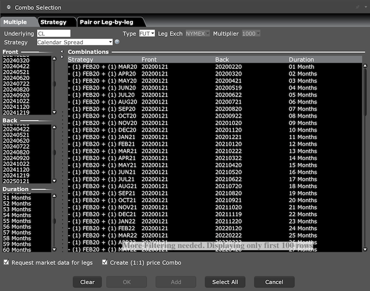
Traders can also speculate on the future shape of the oil curve of a single crude oil type.
Example WTI crude oil spread combination trade opportunities through Interactive Brokers:
Because certain commodities compete with and are interchangeable with each other – e.g., corn and soybean meal as pig, chicken, and cattle feed – if one becomes too expensive relative to another, a trader might believe that they can go long the cheap feed and short the expensive feed.
Or traders might want to trade one raw product versus the refined version of the product. In energy, these types of spreads are called “crack spreads”. In agricultural products, they are referred to as “crush spreads”.
Examples
– Crude oil vs. heating oil
– Crude oil vs. gasoline
– Crude oil vs. heating oil + gasoline
– Soybeans vs. soybean oil
– Soybeans vs. soybean meal
– Soybeans vs. soybean oil + soybean meal
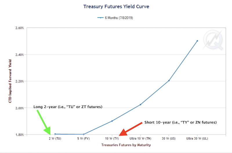
For those who trade US Treasuries, inter-commodity spreads help to efficiently execute trades on the shape of the yield curve.
For example, if there is an inversion or tight spread between the 2-year and 10-year Treasury, a trader might believe that this is unsustainable (the 10-year Treasury should compensate more due to duration risk). Accordingly, they might want to short the 10-year Treasury, betting on a higher yield, and go long the 2-year Treasury.
They could do this with the cash bonds, but typically traders will try to do it more efficiently through the futures markets. They can also get more leverage and do it in a single transaction.
The CME Globex code for the 10-year / 2-year spread is TUT. To account for contract size and duration differential between the 2-year (ZT futures) and 10-year (ZN futures), the TUT spread includes two ZT contracts for every one ZN contract.
This can also be traded for different contract maturities.
Fed funds futures and eurodollars both fundamentally follow the same market – the fed funds rate set by the US Federal Reserve. This provides relative value opportunities for those who trade rates.
The CME Group includes its own Treasuries inter-commodity spread analytics on its website. The same ICS analytics are available for interest rate futures products as well.
Inter-commodity spread products available
Below is a selection of inter-commodity spreads geared toward interest rate, Treasuries, and swap futures products.
It includes the following information:
– Spread (i.e., which products are involved)
– Spread ratio (to account for differentials between contract size and volatility to make the spread bet as fair as possible)
– CME Globex code (identifies the spread and accordingly the trade being placed if selected)
– Bloomberg code (if you have a Bloomberg terminal, this is the code you can enter to view the current spread)
| Spread | Spread ratio* | CME Globex code
(September 2019 Contract Example) |
Bloomberg code |
| STIRS | |||
| Fed Funds vs. Eurodollars | 6:10 | ZQV9X9-GEU9 | FFED Comdty |
| SOFR 3-Month vs. Eurodollars | 1:1 | SR3U9-GEU9 | SFRED Comdty |
| SOFR 1-Month vs. Fed Funds | 1:1 | SR1U9-ZQU9 | SERFF Comdty |
| SOFR 1-Month vs. SOFR 3-Month | 6:10 | SR1 V9X9-SR3U9 | SERSFR Comdty |
| Fed Funds vs. SOFR 3-Month | 6:10 | ZQ V9X9-SR3U9 | FFSFR Comdty |
| Treasuries | |||
| 2-Year T-Note vs. 5-Year T-Note | 5:4 | TUF 05-04 U9 | |
| 2-Year T-Note vs. 5-Year T-Note | 3:2 | TAF 03-02 U9 | |
| 2-Year T-Note vs. 10-Year T-Note | 2:1 | TUT 02-01 U9 | |
| 5-Year T-Note vs. 10-Year T-Note | 3:2 | FYT 03-02 U9 | |
| 5-Year T-Note vs. T-Bond | 4:1 | FOB 04-01 U9 | |
| 10-Year T-Note vs. T-Bond | 5:2 | NOB 05-02 U9 | |
| T-Bond vs. Ultra T-Bond | 3:2 | BOB 03-02 U9 | |
| Eris Swap futures | |||
| 2-Year vs. 3-Year Eris Swap futures | 3:2 | ETR 03-02 U19 | |
| 2 Year vs. 7 Year Eris Swap futures | 3:1 | ETV 03-01 U19 | |
| 2-Year vs. 10-Year Eris Swap futures | 4:1 | ETN 04-01 U19 | |
| 4-Year vs. 5-Year Eris Swap futures | 5:4 | EOF 05-04 U19 | |
| 5-Year vs. 7-Year Eris Swap futures | 4:3 | EFV 04-03 U19 | |
| 5-Year vs. 10-Year Eris Swap futures | 2:1 | EFN 02-01 U19 | |
| 7-Year vs. 10-Year Eris Swap futures | 4:3 | EVN 04-03 U19 | |
*Price and quantity ratios are expected to remain unchanged absent substantial changes in the marketplace
Spread trades and the dangers of extrapolating the past
As mentioned, inter-commodity spreads are chiefly used in the context of relative value or spread trades (and sometimes arbitrage, if they can truly be called that).
However, relative value trades are often applied using assumptions based on the past that may not necessarily hold up in the future.
One example is Brent crude versus WTI crude. Brent, post-2010, has traded at a premium to WTI. This is primarily a function of higher transportation and storage costs given it’s produced in the North Sea away from major refineries.
When the spread becomes excessively tight or too wide, some traders will believe this to be a mispricing to exploit. But this relationship changes over time for logical reasons (e.g., changes in pipelines). If a trader isn’t on top of why the relationship is different and is simply extrapolating the past when the future is different, a relative value trade is probably going to go poorly, or at least see its outcome reduced down the luck associated with any other speculative bet.
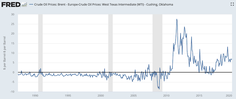
(Source: US Energy Information Administration)
A trader might look at this graph and believe that a long WTI / short Brent trade might be a good idea if the spread got to $10 or more. Right now, if the spread went there for no fundamentally driven reason, that would be a reasonable trade idea. But if the future relationship changes, all of that goes out the window.
It’s a similar thing with chart analysis that’s relied on heavily by beginning traders. Entering trades based on chart patterns that were formed based on previous price action lacks much in the way of deep logic. There’s a lack of getting at the underlying cause and effect relationships of what causes prices to move, deferring to the simplicity of the (bad) assumption that what happened in the past is likely to continue in the future.
It can be said about anything. If one is a believer in forward price/earnings ratios to identify stocks or stock indices that are cheap or expensive, you might think Hong Kong or Russian stocks are cheap trading at forward multiples of 10 or less compared to US stocks trading at a multiple of 19.
But valuation or notional equilibrium value is unreliable as an indicator of future price movement. It also fails to account for the very different sectoral distributions (US stocks have a much larger allocation to tech than Hong Kong equities, which are dominated by financials) and governance disparities (e.g., Russian equities have a large proportion of state-run enterprises), which cause structural discrepancies in price/earnings differentials.
Relative value trades are also essentially synthetic short gamma trades. This means that when anticipating a spread to go a certain way, you probably expect only a certain amount of movement before the reward/risk becomes less attractive. At the same time, spread trades can also go very against you if the nature of the relationship has changed, due to a lack of liquidity, the use of too much leverage, an uptick in broader market volatility that causes spreads to widen, among other reasons.
And because these trades are typically done with futures contracts, which require low collateral outlay relative to the amount of notional exposure. In other words, the leverage is high. So, if you bet wrong, the results can be devastating.
The case of Long-Term Capital Management
The hedge fund Long-Term Capital Management (LTCM) became a huge systemic risk to the global financial system in the late 1990s by leveraging relative value trades. The original core strategy of the fund relied on trades predicting the convergence of the spread between “off-the-run” and “on-the-run” bonds in fixed income futures markets. Because the spread involved in most relative value and arbitrage trades is so small (particularly in the case of the latter), the fund leveraged up many times to generate the high annualized returns (over 40 percent) in its first few years.
Because LTCM was successful at exploiting these relative value and arbitrage opportunities, and the intellectual capital of their team was so strong (which included Nobel Laureates, among many other accomplished people), more investors wanted to be part of their fund.
This caused their assets under management to grow at the same time these opportunities were being arbitraged out of the market, both by themselves and others looking to emulate them. After all, they were considered to be on the forefront of investing at the time.
To obtain their desired results, they increased their leverage and were forced to allocate capital to markets and trades that were beyond the initial scope of their expertise.
They ventured into merger and acquisition arbitrage, directional bets, and applied strategies to emerging markets after previously focusing mostly in more liquid developed markets.
Going into 1998, even though its assets under management were $5 billion (high, but not uncommon), its notional exposure to the markets was well over $1 trillion (200x-250x leverage). That was over 10 percent of US GDP at the time. Of course, when leveraged 200x, that means that a mere 50-bp swing in the fund’s equity position would wipe out the entire capital base.
That summer, markets were volatile due to the fallout from currency crises from developing Asian markets from the year before, and Russia was nearing a point where it would devalue its currency and eventually default on its debt. On top of that, Salomon Brothers, one of LTCM’s counterparties, decided to exit the arbitrage business, which caused a widening in the spreads of LTCM’s trades.
Russia’s problems led to a reduction in “risk on” trades and a flight into global safe haven assets (e.g., US Treasuries, gold, yen). This caused a further widening of the spreads on LTCM’s relative value and arbitrage trades.
Moreover, the run-up in tech shares that would soon become the story of the late 1990s. The NASDAQ bubble was starting to begin, where long-term fundamental valuations of tech companies were misunderstood or ignored. After Alan Greenspan’s “irrational exuberance” speech on December 5, 1996, warning of high valuations in the equity markets and excess speculation, the NASDAQ would eventually quadruple its valuation.
Due to a confluence of factors where the markets “weren’t acting as they were supposed to act”, LTCM’s losses began to stack up.
Because of the size of the fund’s positions, compounded by its injudicious use of leverage, liquidating them was not feasible. The fund’s counterparties also began to understand the scope of LTCM’s problems – which mean their problems – which, in turn, led to the hedging of counterparty risk specific to themselves. This dispersed LTCM’s issues to more and more entities in the financial system and led to even worse problem’s for LTCM itself.
To avoid default, and potential systemic issues for the economy at large, the Federal Reserve Bank of New York stepped in to negotiate a bailout package with LTCM’s creditors.
LTCM had assembled an incredible team of very bright people. But it illustrates the severe inadequacy of bad assumptions in risk management, such as the inappropriate use of using the past to inform the future.
Markets are not like a chess game where you can look at what worked in the past, and what can work based on a fixed set of rules within the context of a closed system, and expect it to work like that in perpetuity. That type of extrapolation can be logical where you know previous environments will work exactly like future environments. The financial markets are not like that.
LTCM’s risk management models assessed their odds of a blowup as 1-in-6 billion. But market history is full of seemingly low probability events that occurred due to poor estimations of their actual probabilities. In LTCM’s case, despite the intellectual capacity of their team, they failed to consider that the correlations of their positions became increasingly linked for no other reason than the fact that they owned them. If you become a material portion of your market, that can become a problem because of the liquidity premium associated with that. The same happened when the Hunt brothers attempted to corner the silver market in the late 1970s and early 1980s.
In reality, the notion of a truly risk-free arbitrage bet is non-existent. On a very small scale with premium execution, it might not be an issue.
But when the relative value and arbitrage positions LTCM was trying to exploit were very small, the position sizes were magnified in a dangerous way to achieve the desired return on equity.
This put the fund at risk to its counterparties’ financing fees and its willingness to provide financing. When market liquidity decreased and the spreads widened, their mark-to-market losses increased, they were stuck and had nowhere to go.
Choosing the appropriate asset classes to trade inter-commodity spreads
Inter-commodity spreads are heavily reserved for interest rates, bonds, and commodities.
Relative value trades can be done with stocks on a broker like IBKR.
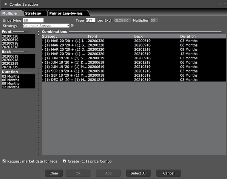
(Example of trading equity index spreads through ES futures on Interactive Brokers)
But they are less common.
Interest rates, bonds, and commodities are more concrete and less prone to distorted perceptions of value. Stocks can get too high or too low because people tend to refer to the recent past to inform the future. Accordingly, they buy (or sell) simply because the price has recently gone up (or down). Financial assets are one of the few things in life that seemingly become more psychologically attractive to buy when they go up in price and scoffed at as worse things to buy when they decrease in price.
The values of more speculative instruments can be very inconclusive at any point in time. However, with something like cattle futures or lean hogs, they are ultimately priced based on what people are willing to pay for the meat in stores, supermarkets, and other assorted retailers.
The price of a pig is simply the price of a piglet (which is cheap), with a lot of feed added to it (mostly corn and soybean meal).
Because corn and soybean meal are interchangeable with each other and compete for a lot of the same land space, the markets for the two are inter-related as well.
That comes with calculations regarding factors specific to them:
– planted acreage and expected yields
– rainfall and temperature and their feed-through into yield estimates and harvest sizes
– carrying costs
– livestock inventories by weight and location
– feed cost for individual livestock animals
– the rate at which various livestock animals gain weight
– seasonal variations in the amounts slaughtered
– dressing percentage (meat yielded from a carcass expressed as a percentage)
– retailer and meatpacker margins
– consumer preferences for various cuts of meat
Based on this information, traders can determine how much corn and soybean meal will be consumed (demand), how much corn and soybean meal will be produced (supply), how much meat will come to the market and compete for consumer dollars, and how meat will be likely to be priced to maximize the profits of retailers and meatpackers.
Then traders will take their analysis, look at how that compares to what’s already in the price, determine what to do about it – e.g., do nothing, take a directional trade, take a spread trade, what instrument to use (e.g., individual futures, inter-commodity spreads), and how to size the position within the context of their portfolio, and so forth.
You can do similar types of analysis in equities but, as alluded to, the distortions in stock prices are very high because their cash flows are theoretically perpetual.
By contrast, in commodities, there are settlement prices. The same goes for bonds, which typically have a set date at which they mature. If you’re betting on interest rates, particularly those that are set to a specific level at a certain date by a central bank, whether you win or lose that trade will be based on what policymakers do (or how well you trade the price movement and perceptions of what the central bank will do before the contract settles).
Conclusion
Inter-commodity spreads (ICS) are mostly traded within the context of relative value or spread trades. It should be noted that spread trades are not guarantees and should not be conflated with true arbitrage trades where settling a price differential is straightforward.
Traders should be wary of extrapolating the past to inform the future. Because the corn-wheat spread reaches a certain level beyond its historical norm doesn’t mean that it’s fundamentally not justified. And even if the fundamentals don’t support the relative pricing, it is dangerous to assume that the market will begin to discount that insight for you. Markets can move against you for a long time even if you’re ultimately right. Leverage only magnifies the problem.
Inter-commodity spreads are a valuable tool that traders can use, but they are more advanced and require a deep understanding of the cause and effect relationships that move the particular market(s) involved and how they can be utilized to profit off a pricing differential.